Semantic Approximation for Reducing Code Bloat in Genetic Programming

(1)

Journal Pre-proof

Semantic Approximation for Reducing Code Bloat in Genetic Programming Quang Uy Nguyen, Thi Huong Chu

PII: S2210-6502(20)30382-5

DOI: https://doi.org/10.1016/j.swevo.2020.100729 Reference: SWEVO 100729

To appear in: Swarm and Evolutionary Computation BASE DATA Received Date: 15 January 2019

Revised Date: 10 March 2020 Accepted Date: 28 May 2020

Please cite this article as: Q.U. Nguyen, T.H. Chu, Semantic Approximation for Reducing Code Bloat in Genetic Programming, Swarm and Evolutionary Computation BASE DATA, https://doi.org/10.1016/

j.swevo.2020.100729.

This is a PDF file of an article that has undergone enhancements after acceptance, such as the addition of a cover page and metadata, and formatting for readability, but it is not yet the definitive version of record. This version will undergo additional copyediting, typesetting and review before it is published in its final form, but we are providing this version to give early visibility of the article. Please note that, during the production process, errors may be discovered which could affect the content, and all legal disclaimers that apply to the journal pertain.

(2)

Semantic Approximation for Reducing Code Bloat in Genetic Programming

Quang Uy Nguyen^a, Thi Huong Chu^a,∗

aFaculty of IT, Le Quy Don Technical University, Hanoi, Vietnam

Abstract

Code bloat is a phenomenon in Genetic Programming (GP) characterized by the increase in individual size during the evolutionary process without a corresponding improvement in fitness. Bloat negatively affects GP performance, since large individuals are more time consuming to evaluate and harder to interpret. In this paper, we propose two approaches for reducing GP code bloat based on a semantic approximation technique. The first approach replaces a random subtree in an individual by a smaller tree of approximate semantics.

The second approach replaces a random subtree by a smaller tree that is semantically approximate to the desired semantics. We evaluated the proposed methods on a large number of regression problems. The experimental results showed that our methods help to significantly reduce code bloat and improve the performance of GP compared to standard GP and some recent bloat control methods in GP. Furthermore, the performance of the proposed approaches is competitive with the best machine learning technique among the four tested machine learning algorithms.

Keywords: Genetic Programming, Semantic Approximation, Code Bloat

∗Thi Huong Chu; Mobile: 84-973080942

Email addresses: quanguyhn@gmail.com(Quang Uy Nguyen),huongktqs@gmail.com (Thi Huong Chu )

(3)

1. Introduction

Genetic Programming (GP) is an evolutionary method to find solutions in the form of computer programs, for a problem [20]. A GP system is started by initializing a population of individuals. The population is then evolved for a number of generations using genetic operators such as crossover and mutation.

At each generation, the individuals are evaluated using a fitness function, and a selection schema is used to choose better individuals to create the next population. The evolutionary process is continued until a desired solution is found or when the maximum number of generations is reached.

Although GP has been successfully applied to many real-world problems, it is still not widely accepted as other machine learning approaches e.g. Support Vector Machines or Linear Regression [27]. This is due to some important short- comings of GP such as its poor local structure, ill-defined fitness landscape and code bloat [34]. Among them, bloat phenomenon is one of the most studied problems. Bloat happens when individuals grow too large without a corresponding improvement in fitness [40, 52]. Bloat causes several problems to GP: the evolutionary process is more time consuming, it is harder to interpret the solutions, and the larger solutions are prone to overfitting. To date, many techniques have been proposed to address bloat. These techniques range from limiting individual size to designing specific genetic operators for GP [8, 11, 14, 25, 26, 36, 42, 43].

In this paper, we present a novel approach to control GP bloat, that leverages the previous studies [8, 9]. Our methods are based on theSemantic Approxima- tion Technique(SAT) that allows to grow a small tree of similar semantics to a target semantic vector. Using SAT, we proposed two methods for lessening GP code bloat. The first method isSubtree Approximation(SA) in which a random subtree is selected in an individual and this subtree is replaced by a small tree of approximate semantics. The second method isDesired Approximation (DA) where the new tree is grown to approximate the desired semantics of the subtree instead of its semantics. The performance of the bloat control strategies is examined on a large set of regression problems employing the benchmark and

(4)

the UCI problems. We observe that the new methods help to significantly reduce code growth and improve the generalization ability of the evolved solutions when compared to standard GP and the state of the art methods for controlling code bloat in GP. Moreover, the proposed methods are also better than three popular machine learning models and competitive with the fourth one.

The main contribution of this paper is the demonstration how the idea of semantic approximation (presented in Section 4) can be utilized to reduce code growth in GP. Comparing to [8, 9] where we originally proposed this technique, here we present a generalized version of semantic approximation and a better technique for controlling code bloat. Moreover, the proposed methods are thoroughly examined and compared with a number of GP and non-GP systems on a wider range of regression problems.

The remainder of this paper is organized as follows. In the next section, we present the background of the paper. Section 3 reviews the related work on managing code bloat in GP. The semantic approximation technique and two strategies for lessening code bloat are presented in Section 4. Section 5 presents the experimental settings adopted in the paper. Section 6 analyses and compares the performance of the proposed strategies with standard GP and some recent related methods. Some properties of our proposed methods are analyzed in Section 7. Section 8 compares the proposed methods with four popular machine learning algorithms. Finally, Section 9 concludes the paper and highlights some future work.

2. Background

This section presents some important concepts used in this paper, including the semantics of a GP individual and the semantic backpropagation algorithm.

2.1. Semantics Definition

When using GP to solve a problem, we are mostly interested in the behavior of the individuals (what they ‘do’). To specify what individual behavior

(5)

is, researchers have recently introduced semantics concept in GP [11, 23, 29].

Formally, the semantics of an individual (program) is defined as follows:

Definition 2.1. Let K= (k1, k2, ...kn)be the fitness cases of the problem. The semanticss(p)of a programpis the vector of output values obtained by running pon all fitness cases.

s(p) = (p(k₁), p(k₂), . . . , p(k_n)), for i= 1,2, . . . , n.

This definition is also calledsampling semantics[48, 49] and it is not a complete description of the behavior of individuals. The semantics of an individual consists of a finite sample of outputs with respect to a set of training values.

Moreover, the definition is only valid for programs whose output is a single real- valued number, as in symbolic regression. However, it is widely accepted and extensively used for designing many new techniques in GP [11, 36, 48].

Over the last few years, semantics has been the intensively studied topic in GP. For a comprehensive review and comparison of various semantic methods in GP, the readers are recommended to see [23]. Usually, semantic methods are integrated into GP for defining the new genetic operators, which can be divided into two types: indirect and direct [23]. Indirect methods achieve desired semantic criteria by sampling and rejection. They alter the syntax of the parents [4, 5, 21, 32, 36, 47, 48, 49]. In contrast, direct methods generate new children with desired semantic criteria which incorporate the complete syntax of their parents without modification [22, 30, 33, 36]. In this paper, we propose a new usage of semantics in GP. Specifically, a technique for generating a new tree that is semantically approximate (similar) to the target semantics is introduced and used for reducing code bloat in two different strategies.

2.2. Semantic Backpropagation

The semantic backpropagation algorithm was proposed by Krawiec and Pawlak [36] to determine the desired semantics for an intermediate node of an individual. The algorithm starts by assigning the target of the problem (the output of the training set) to the semantics of the root node and then propagates

(6)

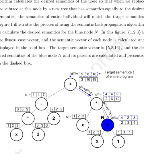
the semantic target backwards through the program tree. At each node, the algorithm calculates the desired semantics of the node so that when we replace the subtree at this node by a new tree that has semantics equally to the desired semantics, the semantics of entire individual will match the target semantics.

Figure 1 illustrates the process of using the semantic backpropagation algorithm to calculate the desired semantics for the blue nodeN. In this figure,{1,2,3}is the fitness case vector, and the semantic vector of each node is calculated and displayed in the solid box. The target semantic vector is{5,8,16}, and the desired semantics of the blue nodeN and its parents are calculated and presented in the dashed box.

Figure 1: An example of calculating the desired semantics of the selected nodeNby using the semantic backpropagation algorithm.

The semantic backpropagation technique is then used for designing several genetics operators in GP [36]. Among these, Random Desired Operator (RDO) is the most effective operator [33, 36]. A parent is selected by a selection scheme, and a random subtreesubT reeis chosen. The semantic backpropagation algorithm is used to identify the desired semantics ofsubT ree. After that, a procedure is called to search in a predefined library of trees for a newT ree that is the most semantically closest to the desired semantics. Finally, newT reeis

(7)

replaced forsubT reeto create a new individual. This operator performs very well on both real-valued and Boolean problems as reported in [33, 36].

3. Related Work

Due to the negative impact of code bloat, many approaches have been proposed to control bloat and lessen its impact on GP performance. Generally, the bloat control methods can be divided into three main groups: constraining individual size, adjusting selection techniques and designing genetic operators.

3.1. Constraining Individual Size

Earlier techniques are often based on limiting the size of individuals to pre- vent bloat [20, 26]. Any offspring with the size or depth above the limits is rejected and replaced by one of its parents. Some later research used the dynamic limits that are derived from the size of the best-so-far individual [42] or from the average size of the population [38, 39]. Overall, these approaches have relatively succeeded in controlling code bloat. However, it is difficult to select an appropriate value of the limits. If the limits are set at too small values, the improvement of fitness values may be prevented.

3.2. Adjusting Selection Techniques

The second approach is to use more than one fitness value in the selection.

The parsimony pressure technique punishes the large individuals in the fitness function or prefers to choose smaller individuals in selection methods. The fitness is a linear combination of the individual size and its fitness value [6, 7], or is assigned a very bad fitness for large individuals in the population [38, 39].

Lexicographic Parsimony Pressure (LPP) [25] compares two random individuals in Boolean and Artificial Ant problems using two criteria: fitness and size. If two individuals have different fitness then the better fitness individual is chosen. Conversely, the smaller individual is selected. Double Tournament [25]

selects individuals using two tournaments: one based on fitness and one based on size. The winners of fitness tournament go on to compete in the tournament

(8)

using size to select the smaller individuals for the mating pool. Biased Multi- Objective Parsimony Pressure method (BMOPP) [35] sorts individuals into a Pareto layer based on the concept of denomination: an individual A dominates an individual B if A is as good as B in all objectives and is better than B in at least one objective. After the Pareto layers have been formed, individuals are selected using tournament selection. The individuals are compared with each other based on their fitness with probability P and based on their respective Pareto layers with probability 1−P.

An extension of LPP is Spatial Structure with Lexicographic Parsimonious Elitism (SS+LPE) [13]. SS+LPE implicitly controls bloat by mapping the population onto a 2D torus and defines a neighborhood relationship between individuals on this topology. At each generation, an individual is mated with one of its neighbors. The offspring is then compared with the parent using LPP to choose the winner for the next generation. Recently, Chu et al. [10, 11] proposed Statistics Tournament Selection with Size (TS-S) for reducing code bloat.

To select the winner in a tournament, TS-S uses a statistical test on the error vector of the sampled individuals. For a pair of individuals, if the test shows that the individuals are different, then the individual with a better fitness value is the winner. Conversely, the individual with smaller size is chosen.

3.3. Designing Genetic Operators

The third approach has received a considerable attention, lately. Alfaro-Cid et al. [1] proposed Prune and Plant (PP) operator that splits an individual into two ones. A random subtree is selected and replaced by a terminal to create the first offspring. The selected subtree is also added to the population as the second offspring. Operator Equalisation (OE) [14] focuses explicitly on controlling the distribution of program sizes at each generation. OE determines a target histogram for the individuals in which the width of the bin determines the size of the programs belonging to the bin, and the height represents the number of individuals in the bin. OE then directs the population to the target distribution by accepting or rejecting each newly created individual into its corresponding

(9)

bin. However, OE is computationally expensive because it requires to generate and reject many individuals that do not fit the desired target distribution.

Silva et al. used a Flat Target Distribution (Flat-OE) [41, 43] to address the shortcoming of OE. In other words, the range of the distribution remains constant throughout the search. Empirical results suggest that Flat-OE can control bloat while maintaining the quality of obtained solutions. Gardner et al. [16] extended OE by using the cutoff point concept and the accept–reject method to adjust the target distribution. The cutoff point is the size of the smallest individual which reaches a certain percentage of the best fitness so far. The bins are then only applied to the individuals of larger size than the cutoff point. Trujillo et al. [46] controlled code bloat by using neat-crossover operator in neat-GP system. This operator first identifies the shared topological structureSij between parents, and then swaps of a single internal node between the parents in S_ij. In this way, offspring maintain the topological structure of their parents. Thus, the size of the resultant tree does not increase after crossover. neat-GP was then extended to neat-GP-LS by integrating with local search [18, 45].

Recently, Fracasso and Zuben [15] proposed Multi-Objective Randomized Similarity Mutation (MORSM) and Multi-Objective Desired Operator(MODO) to avoid the bloating effect in mutation. First, a Restricted Candidate List (RCL) which consists of subprograms that are taken from a predefined library and are not dominated for a given set of objectives (the semantic distance, the individual length) is constructed. Next, a random subtree of a parent is replaced by a random subprogram chosen in RCL. In MORSM, RCL is built using the objective that is the semantic distance between the subtree and the subprogram while in MODO, the objective is the semantics distance between the desired semantics [36] at the subtree and the subprogram. In the next section, we will introduce the semantic approximation technique that allows to generate a new tree of semantically similar to the target semantics. Using this technique, we will propose two new genetic operators for reducing GP code bloat.

(10)

4. Methods

This section presents a new technique for constructing a program that ap- proximates a given semantic vector and two methods for reducing GP code bloat based on that.

4.1. Semantic Approximation

Searching for a tree that is semantically approximate or similar to a target semantic vector has been important in several researches [36, 48]. Nguyen et al. [48] searched for a pair of semantically similar subtree by repeatedly sampling from two parents. Pawlak and Krawiec [36] found a tree that is semantically closest to the desired semantics from a predefined library. In this paper, we introduce a novel approach to generate a tree of approximate semantics to the target semantics. This approach is called the Semantic Approximation Tech- nique (SAT).

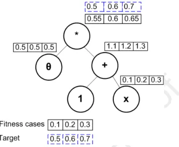
LetS= (s₁, s₂, ..., s_n) be the target semantics, then the objective of SAT is to grow a tree in the form: newT ree=θ·sT ree (sT ree is a small randomly generated tree) so that the semantics of newT ree is as close to S as possible.

LetQ= (q1, q2, ...qn) be the semantics ofsT ree, then the semantics ofnewT ree isP = (θ·q1, θ·q2, ..., θ·qn). To approximate S, we need to findθso that the squared Euclidean distance between two vectorsS andP is minimal. In other words, we need to minimize functionf(θ) =PN

i=1(θ·qi−si)² with respect to θ. The quadratic functionf(θ) achieves the minimal value at θ^∗ calculated in Equation 1:

θ^∗= PN

i=1qisi

PN

i=1q_i² (1)

After finding θ^∗, newT ree = θ^∗ ·sT ree is grown, and this tree is called the approximate tree of the semantic vector S. Figure 2 presents an example of growing a tree in the form: newT ree= θ·sT ree where sT ree = (1 +X) using SAT. In this figure,X ={0.1,0.2,0.3}is the fitness cases of the problem, S={0.5,0.6,0.7}is the target semantics. Using Equation 1 we haveθ^∗≈0.5.

(11)

Figure 2: An example of Semantic Approximation

Compared to the previous techniques [36, 48], SAT has some advantages.

First, SAT is easier to implement and faster to execute than the techniques in [36, 48]. Subsequently, GP systems based on SAT will run faster. Second, GP operators using SAT will create the population of higher diversity than the operators that only search for the subtree in other individuals [48] or from a predefined library [36]. Thus, SAT-based operators may achieve better performance than SSC [48] and RDO [36]. Last but not least, the size ofnewT reecan be constrained by limiting the size ofsT ree, and this will be used for designing two approaches to reduce GP code bloat in the next subsections.

4.2. Subtree Approximation

Based on SAT, we propose two techniques for reducing code bloat in GP.

The first technique isSubtree Approximation (shortened as SA). At each generation, after applying genetic operators to generate the next population, k%

largest individuals in the population are selected for pruning. Next, a random subtree is chosen in each selected individual. This subtree is then replaced by an approximate tree of smaller size. Algorithm 1 presents this technique in detail.

(12)

In Algorithm 1, function InitializeP opulation() creates an initial population using the ramped half-and-half method. FunctionGenerateN extP op(Pi−1) generates the template population using crossover and mutation. The next step selectsk% of the largest individuals in the template population (P⁰i) and stores them in a pool. The loop after that is used to simplify the individuals in the pool.

Algorithm 1:Subtree Approximation Input: P op Size:N,N um P rune:k%

i←−0

P0←−InitializeP opulation()

Estimate fitness of all individuals in P⁰ repeat

i←−i+ 1

P⁰i←−GenerateN extP op(Pi−1)

pool←−getk% of the largest individuals ofP⁰i

Pi←−P⁰i−pool foreachI⁰∈pool do

subT ree←−RandomSubtree(I⁰) S←−Semantics(subT ree)

newT ree←−SemanticApproximation(S) I←−Substitute(I⁰, subT ree, newT ree) Pi←−Pi∪I

Estimate fitness of all individuals in Pi

until Termination condition met

For each individualI⁰ in the pool, a random subtreesubT reeinI⁰is selected using functionRandomSubtree(I⁰), and a small treesT reeis randomly generated¹. The semantics ofsubT reeis calculated and assigned toS(Sbecomes the

1To reduce bloat, the size ofsT reeneeds to be smaller than the size ofsubT ree−2. If this condition is not satisfied, the process of selectingsubT reeand generatingsT reeis repeated.

(13)

target semantics) with functionSemantics(subT ree). AnewT ree=θ·sT reeis grown to approximateSin functionSemanticApproximation(S). Finally, indi- vidualI⁰ is simplified to form individualI by replacingsubT reewithnewT ree.

Individual (I) is added to the next generation,Pi. The population at the gen- erationiis then evaluated using the fitness function, and the whole process is repeated until the termination condition meets.

4.3. Desired Approximation

The second technique, Desired Approximation (DA), attempts to achieve two objectives simultaneously: lessening GP code bloat and enhancing its ability to

Algorithm 2:Desired Approximation Input: P op Size:N,N um P rune:k%

i←−0

P0←−InitializeP opulation()

Estimate fitness of all individuals in P0

repeat i←−i+ 1

P⁰i←−GenerateN extP op(Pi−1)

pool←−getk% of the largest individuals ofP⁰i

Pi←−P⁰i−pool foreachI⁰∈pool do

subT ree←−RandomSubtree(I⁰) D←−DesiredSemantics(subT ree) newT ree←−SemanticApproximation(D) I←−Substitute(I⁰, subT ree, newT ree) Pi←−Pi∪I

Estimate fitness of all individuals in Pi

until Termination condition met

If no pair ofsubT reeandsT reeis found after 100 trials, individualI⁰is added to the next generation.

(14)

fit the training data. DA is similar to RDO [36] in which it first calculates the desired semantics for a randomly selected subtree in a large individual using the semantic backpropagation algorithm [36]. However, instead of searching for a tree in a predefined library, DA uses SAT to grow a small tree that is semantically approximate to the desired semantics. Algorithm 2 thoroughly describes DA.

The structure of Algorithm 2 is very similar to that of SA. The main difference is in the second loop. First, the desired semantics ofsubT reeis calculated instead the semantics ofsubT ree. Second, newT reeis grown to approximate the desired semantics D of subT ree instead of its semantics S. By replacing subT reeby a newT reethat is semantically approximate to the desired semantics, it is predicted that the individual will be closer to the optimal value.

5. Experimental Settings

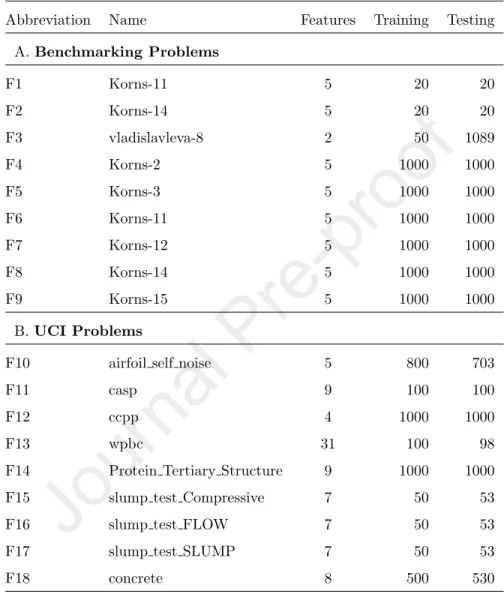
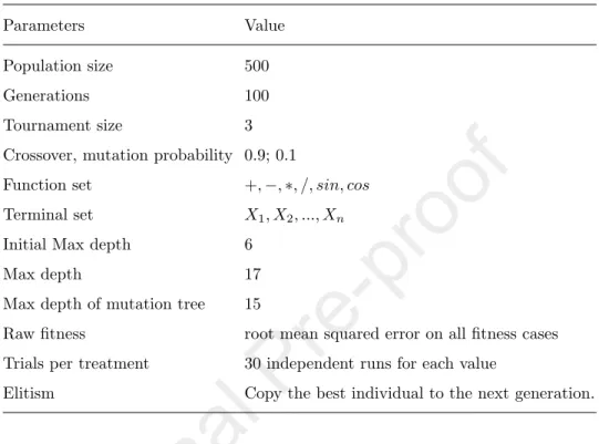
We tested SA and DA on nine GP benchmark problems recommended in the literature [53], and an additional nine real problems are taken from UCI machine learning repository [3]. The abbreviation, the name, number of features, number of training and testing samples of each problem are presented in Table 1. The GP parameters used in our experiments are shown in Table 2. The raw fitness is the root mean squared error on all fitness cases. Therefore, smaller values are better. For each problem and each parameter setting, 30 runs were performed.

We compared SA and DA with standard GP (referred to as GP), Prune and Plant (PP) [1], Statistics Tournament Selection with Size (TS-S) [11] and Ran- dom Desired Operator (RDO) [36]. PP is probably the most similar technique to SA, RDO is the inspiration for DA and TS-S is the most recently proposed bloat control method. The probability of PP operator was set to 0.5. This is the value for the best performance of PP [1, 2]. For RDO, we used a predefined library of 1000 subprograms with max depth of 2.

For SA and DA, 10% and 20% of the largest individuals in the population were selected for pruning. The corresponding versions were shortened as SA10,

(15)

Table 1: Problems for testing the proposed methods

Abbreviation Name Features Training Testing

A. Benchmarking Problems

F1 Korns-11 5 20 20

F2 Korns-14 5 20 20

F3 vladislavleva-8 2 50 1089

F4 Korns-2 5 1000 1000

F5 Korns-3 5 1000 1000

F6 Korns-11 5 1000 1000

F7 Korns-12 5 1000 1000

F8 Korns-14 5 1000 1000

F9 Korns-15 5 1000 1000

B.UCI Problems

F10 airfoil self noise 5 800 703

F11 casp 9 100 100

F12 ccpp 4 1000 1000

F13 wpbc 31 100 98

F14 Protein Tertiary Structure 9 1000 1000

F15 slump test Compressive 7 50 53

F16 slump test FLOW 7 50 53

F17 slump test SLUMP 7 50 53

F18 concrete 8 500 530

SA20, DA10 and DA20. The newT ree was grown from sT ree with the max depth of 2². Moreover, a dynamic version of SA (shortened as SAD) and DA

2This value was selected for the good performance of SA and DA. The experimental results with the max depth=1,3 and 4 are presented in the supplement 1 of the paper at https://github.com/chuthihuong/SemanticApproximation.

(16)

Table 2: Evolutionary parameter values

Parameters Value

Population size 500

Generations 100

Tournament size 3

Crossover, mutation probability 0.9; 0.1

Function set +,−,∗, /, sin, cos Terminal set X1, X2, ..., Xn

Initial Max depth 6

Max depth 17

Max depth of mutation tree 15

Raw fitness root mean squared error on all fitness cases Trials per treatment 30 independent runs for each value

Elitism Copy the best individual to the next generation.

(referred to as DAD) was also tested in which the individuals with the size greater than the average of the population are selected for pruning.

The source code of all tested methods are available for download³. All techniques were implemented in Java. Moreover, the same computing platform (Operating system: Windows 7 Ultimate (64bit), RAM 16.0GB, IntelCore TM i7-4790 CPU@3.60GHz) was used in every experiment in this paper.

For the statistical test, we implemented the Kruskal-Wallis test [28, 12] with the confidence level of 95% on the results of 30 runs. This test does not require the distributions of variables in questions to be normal and detect differences in treatments across multiple approaches. If the Kruskal-Wallis test shows that at least one method is significantly different from the others, we conducted a post hoc analysis with Dunn’s Test. p valuesare adjusted using the Benjamini-

3https://github.com/chuthihuong/SemanticApproximation

(17)

Hochberg procedure. In all tables in Section 6, if the test shows that a method is significantly better than GP, this result is marked + at the end. Conversely, if it is significantly worse than GP, this result is marked - at the end⁴. Moreover, if the result of a method is better than GP, it is printed bold face, and if it is the best value, it is printed underline.

6. Performance Analysis

This section analyses the performance of the proposed methods using four popular metrics: training error, testing error, solution size and running time.

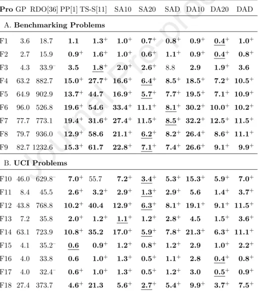
6.1. Training Error

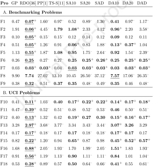
Training error is useful for analysing the learning process of GP. The mean of the best fitness values in the training process across 30 runs is presented in Table 3. The table shows that RDO achieved the smallest training error on most tested problems. This is not surprising since the main objective of RDO is to improve the training error [36]. Among four methods for reducing code bloat (PP, TS-S, SA and DA), PP is the worst. The training error of PP is always much higher than that of the others. TS-S also does not improve the training error compared to GP. The mean best fitness of TS-S is slightly greater than that of GP on most problems. This result is consistent with the result in the previous work [10].

Conversely, the training error of SA and DA is often better than that of GP, PP and TS-S. Comparing between three configurations of SA and DA, we can see that SA10 and DA10 are better than the two other configurations. The training error of DA10 is better than that of GP on all tested problems, and the training error of SA10 is better than that of GP on 12 problems. This result is very impressive since the previous researches showed that bloat control methods often negatively affect the ability of GP to fit the training data [10, 46].

4The p values of the Kruskal-Wallis test with the post hoc analysis are presented in the supplement 2 of the paper at https://github.com/chuthihuong/SemanticApproximation.

(18)

To understand why SA and DA improve the training error of GP while other techniques for controlling bloat are often failed to do so, we measured the percentage of the pruning operator in PP, SA and DA that generates the offspring having better fitness than their parents. This value is calculated in

Table 3: Mean of the best fitness: bold face is better than GP, underline is the best result, + is significantly better than GP, - is significantly worse than GP

Pro GP RDO[36] PP[1] TS-S[11] SA10 SA20 SAD DA10 DA20 DAD A.Benchmarking Problems

F1 0.47 0.07⁺ 1.60^– 0.97^– 0.52 0.89^– 1.30^– 0.41 0.97^– 1.17^– F2 1.91 0.06⁺ 4.45^– 1.79 1.08⁺ 2.33 4.12^– 0.96⁺ 2.20 3.58^– F3 0.10 0.05⁺ 0.15^– 0.15^– 0.12 0.14^– 0.12 0.09 0.12 0.11 F4 0.51 0.05⁺ 1.26^– 0.91 0.06⁺ 0.83 1.88^– 0.13⁺ 0.37⁺ 1.04 F5 1.13 0.55⁺ 1.87^– 1.08 0.95 1.75^– 2.64^– 0.92 1.54^– 2.39^– F6 0.26 0.25 0.27^– 0.27^– 0.25 0.25⁺ 0.26⁺ 0.25 0.25⁺ 0.25⁺ F7 0.03 0.03⁺ 0.03⁺ 0.04^– 0.03 0.03⁺ 0.03⁺ 0.03 0.03⁺ 0.03⁺ F8 9.90 7.74 27.02^– 13.10 10.45 26.50^– 37.12^– 7.57 17.06^– 26.35^– F9 0.38 0.32 0.51^– 0.37 0.35 0.48^– 0.49^– 0.35 0.46 0.48^–

B.UCI Problems

F10 0.41 0.11⁺ 1.03^– 0.40 0.17⁺ 0.22⁺ 0.22⁺ 0.14⁺ 0.17⁺ 0.18⁺ F11 0.47 0.39⁺ 0.52^– 0.51^– 0.48 0.52^– 0.53^– 0.46 0.50^– 0.51^– F12 0.40 0.13⁺ 1.32^– 0.42 0.19⁺ 0.27 0.30 0.15⁺ 0.16⁺ 0.17⁺ F13 3.28 2.97⁺ 3.68^– 3.77^– 3.34 3.43^– 3.44^– 3.07⁺ 3.26 3.29 F14 0.17 0.17⁺ 0.18^– 0.17 0.17 0.18^– 0.18^– 0.17⁺ 0.17 0.17 F15 0.82 0.22⁺ 1.20^– 0.94 0.65⁺ 0.87 0.98 0.45⁺ 0.52⁺ 0.57⁺ F16 1.68 0.88⁺ 2.05^– 1.93^– 1.70 1.99^– 2.05^– 1.51⁺ 1.83 1.93^– F17 0.91 0.56⁺ 1.19^– 1.13^– 0.90 1.11^– 1.11^– 0.84 1.01 1.04^– F18 0.53 0.28⁺ 0.89^– 0.57 0.50 0.64^– 0.66^– 0.41⁺ 0.55 0.61^–

(19)

Equation 2

Pbetter =N_B NP

(2) in which N_P is the number of the offspring that are generated by PP, SA or DA, andN_B is the number of the offspring that is better than its parent. The value across 30 runs was averaged and shown in Table 4.

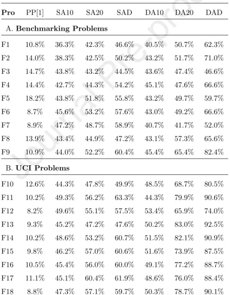
Table 4: Average percentage of better offspring

Pro PP[1] SA10 SA20 SAD DA10 DA20 DAD

A. Benchmarking Problems

F1 10.8% 36.3% 42.3% 46.6% 40.5% 50.7% 62.3%

F2 14.0% 38.3% 42.5% 50.2% 43.2% 51.7% 71.0%

F3 14.7% 43.8% 43.2% 44.5% 43.6% 47.4% 46.6%

F4 14.4% 42.7% 44.3% 54.2% 45.1% 47.6% 66.6%

F5 18.2% 43.8% 51.8% 55.8% 43.2% 49.7% 59.7%

F6 8.7% 45.6% 53.2% 57.6% 43.0% 49.2% 66.6%

F7 8.9% 47.2% 48.7% 58.9% 40.7% 41.7% 52.0%

F8 13.9% 43.4% 44.9% 47.2% 43.1% 57.3% 65.6%

F9 10.9% 44.0% 52.2% 60.4% 45.4% 65.4% 82.4%

B.UCI Problems

F10 12.6% 44.3% 47.8% 49.9% 48.5% 68.7% 80.5%

F11 10.2% 49.3% 56.2% 63.3% 44.3% 79.9% 90.6%

F12 8.2% 49.6% 55.1% 57.5% 53.4% 65.9% 74.0%

F13 9.3% 45.2% 47.2% 47.6% 50.2% 83.0% 92.5%

F14 10.2% 48.6% 53.2% 60.7% 51.5% 82.1% 90.9%

F15 9.8% 46.2% 57.0% 60.6% 51.6% 73.9% 87.5%

F16 10.5% 45.4% 56.0% 60.0% 49.1% 77.2% 88.7%

F17 11.1% 45.1% 60.4% 61.9% 48.6% 76.0% 88.4%

F18 8.8% 47.3% 57.1% 59.7% 50.3% 78.7% 90.1%

(20)

The table shows that PP hardly generates better offspring compared to their parents. This value of PP is only from 10% to 15%. In contrast, this value of SA and DA is much higher (from 40% to 90%). Moreover, we can see that DA generates better offspring more frequently than SA. This is reasonable since DA used the semantic backpropagation algorithm in [36] to improve its fitness.

Comparing between three versions of SA and DA, we can see that, the value of SAD and DAD are better than the value of SA10, SA20, DA10 and DA20, respectively. The reason could be that the mean best fitness of SAD and DAD is often worse than that of the other versions (Table 3). Thus, the probability to improve the fitness of SAD and DAD by using an operator like pruning is higher than of SA10, SA20, DA10 and DA20. Overall, the result in Table 4 helps to partly explain for the better training error of SA and DA compared to the other bloat control methods.

6.2. Generalization Ability

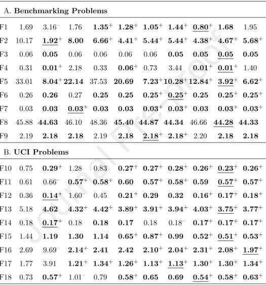
This subsection analyzes the generalization ability of the tested methods through comparing their testing error. In each run, the best solution (the individual with the smallest fitness) was selected and evaluated on the testing data (an unseen data set).

The median of these values across 30 runs was calculated and shown in Table 5. The table shows that all configurations of SA and DA outperform GP on the unseen data. For example, the testing error of SA10 and DA10 is smaller than that of GP on 17 and 16 problems, respectively. Similarly, SA20, SAD, DA20 and DAD are also better than GP on most tested functions. For the other bloat control methods, TS-S is slightly better than GP, and PP is roughly equal to GP. RDO is also better than GP on 14 problems. However, its performance on UCI problems is less convincing.

The results from the Kruskal-Wallis test show that there is a significant difference between the results of the methods in Table 5. Morever, the test also shows that SA and DA are significantly better than GP on most tested problems. SA10, SA20 and SAD are significantly better than GP on 9, 12

(21)

Table 5: Median of testing error: bold face is better than GP, underline is the best result, + is significantly better than GP, - is significantly worse than GP

F1 1.69 3.16^– 1.76 1.35⁺ 1.28⁺ 1.05⁺ 1.44⁺ 0.80⁺ 1.68 1.95 F2 10.17 1.92⁺ 8.00 6.66⁺ 4.41⁺ 5.44⁺ 5.44⁺ 4.38⁺ 4.67⁺ 5.68⁺ F3 0.06 0.05 0.06 0.06 0.06 0.06 0.05 0.05 0.05 0.05 F4 0.31 0.01⁺ 2.18 0.33 0.06⁺ 0.73 3.44 0.01⁺ 0.01⁺ 1.40 F5 33.01 8.04⁺22.14 37.53 20.69 7.23⁺10.28⁺12.84⁺ 3.92⁺ 6.62⁺ F6 0.26 0.26 0.27 0.25 0.25 0.25⁺ 0.25⁺ 0.25 0.25⁺ 0.25⁺ F7 0.03 0.03 0.03⁺ 0.03 0.03 0.03⁺ 0.03⁺ 0.03 0.03⁺ 0.03⁺ F8 45.88 44.63 46.10 48.36 45.40 44.87 44.34 46.66 44.28 44.33 F9 2.19 2.18 2.18 2.19 2.18 2.18⁺ 2.18⁺ 2.20 2.18 2.18

B.UCI Problems

F10 0.75 0.29⁺ 1.28 0.83 0.27⁺ 0.27⁺ 0.28⁺ 0.26⁺ 0.23⁺ 0.26⁺ F11 0.61 0.66^– 0.57⁺ 0.58⁺ 0.60 0.57⁺ 0.58⁺ 0.59 0.57⁺ 0.57⁺ F12 0.36 0.14⁺ 1.60^– 0.45 0.21⁺ 0.29 0.32 0.16⁺ 0.17⁺ 0.18⁺ F13 5.18 4.62 4.32⁺ 4.42⁺ 3.89⁺ 3.91⁺ 3.94⁺ 4.03⁺ 3.75⁺ 3.77⁺ F14 0.18 0.17⁺ 0.18 0.18 0.17 0.18 0.18^– 0.17⁺ 0.17⁺ 0.17⁺ F15 1.44 1.19 1.30 1.14 0.65⁺ 0.87⁺ 0.99 0.52⁺ 0.51⁺ 0.53⁺ F16 2.69 9.69^– 2.14⁺ 2.41 2.42 2.10⁺ 2.04⁺ 2.31⁺ 2.08⁺ 1.97⁺ F17 1.77 3.91 1.21⁺ 1.34⁺ 1.26⁺ 1.13⁺ 1.13⁺ 1.30⁺ 1.30⁺ 1.34⁺ F18 0.73 0.57⁺ 1.01^– 0.79 0.58⁺ 0.65 0.69 0.54⁺ 0.58⁺ 0.63⁺

and 11 problems, respectively. DA is significantly better than GP on 12, 14 and 13 problems corresponding to its three configurations. Conversely, GP is significantly better than SAD on only one problem (F14). TS-S and PP also outperform GP. The testing error of TS-S and PP are significantly better than GP on 5 problems. For RDO, the statistical test shows that it is slightly better

(22)

than GP. RDO is significantly better than GP on 7 problems, it is significantly worse on 3 problems.

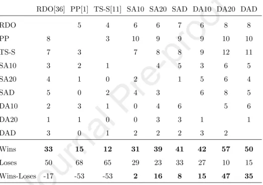
Table 6: Summary of the post hoc analysis of the Kruskal-Wallis test on testing error. Each cell presents the number of problems that the method in a column is significantly better than the method in a row. The number of winning or losing problems of each method in the columns is summed at the bottom of the table.

RDO[36] PP[1] TS-S[11] SA10 SA20 SAD DA10 DA20 DAD

RDO 5 4 6 6 7 6 8 8

PP 8 3 10 9 9 9 10 10

TS-S 7 3 7 8 8 9 12 11

SA10 3 2 1 4 5 3 6 5

SA20 4 1 0 2 1 5 6 4

SAD 5 0 2 4 3 6 8 5

DA10 2 3 1 0 4 6 5 6

DA20 1 1 0 0 3 3 1 1

DAD 3 0 1 2 2 2 3 2

Wins 33 15 12 31 39 41 42 57 50

Loses 50 68 65 29 23 33 27 10 15

Wins-Loses -17 -53 -53 2 16 8 15 47 35

We also summarised the post hoc analysis of the Kruskal-Wallis test to compare the testing error of different bloat control methods. The results are shown in Table 6. In this table, if a method in the columns is significantly better than a method in the rows onk problems,k is presented in the corresponding cell. For example, RDO is significantly better than PP on 8 problems, 8 is presented in the cell at column “RDO” and row “PP”. The result in Table 6 again confirms the good generalization ability of SA and DA. SA and DA are significantly better than RDO, PP and TS-S more frequent than RDO, PP and TS-S are better than SA and DA. For instance, SA20 is significantly better than RDO, PP and TS-S on 6, 9 and 8 problems, respectively, while RDO, PP and

(23)

TS-S are only significantly better than SA20 on 4, 1 and 0 problems. Similarly, DA20 is significantly better than RDO, PP and TS-S on 8, 10 and 12 problems and the vice versa is not true on any problem with TS-S. For RDO and PP, they are significantly better than DA20 on only one problem.

In three rows at the bottom of Table 6, we calculate the total number of winning (significantly better), losing (significantly worse) problems and the difference between winning and losing problems of the method in the columns in Table 5. It can be seen that DA20 is the best method that achieved 57 winning problems and only 10 losing problems, and DAD achieved the second best result with 50 winning problems and 15 losing problems. Among three versions of SA, the table shows that SA20 achieved the best performance. For three methods in the literature, i.e, RDO, PP and TS-S, we can see that their performance is inferior, the number of winning problems is less than the number of losing problems.

Overall, the result in this subsection shows that the performance of SA and DA is more convincing on the testing data compared to the training data.

Moreover, these approaches achieve the best generalization ability compared to all tested methods. Perhaps, the reason for the convincing result of SA and DA on the testing data is that these techniques obtain simple solutions (Table 7) and smaller fitness than the other methods.

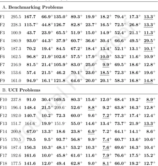
6.3. Solution Size

The main objective for performing bloat control is to reduce the complexity of the solutions. To validate if SA and DA achieve this objective, we recorded the size of the final solution (the individual with the best fitness) in each GP run. These values are then averaged over 30 runs and presented in Table 7.

The table shows that all tested methods find the simpler solutions compared to GP. Among them, SA20, SAD and DA20, DAD often find the smallest solutions. SA10 and DA10 also remarkably reduce the complexity of the solutions but to less extent compared to the other configurations. The solution size of PP is also very small. However, this value is slightly greater than the value

(24)

Table 7: Average size of solutions: bold face is better than GP, underline is the best result, + is significantly better than GP, - is significantly worse than GP

F1 295.5 167.7 66.9⁺135.0⁺ 89.3⁺ 19.9⁺ 18.2⁺ 79.4⁺ 17.3⁺ 13.3⁺ F2 228.3 115.7⁺ 44.8⁺126.7 82.8⁺ 23.7⁺ 16.5⁺ 72.5⁺ 26.8⁺ 13.3⁺ F3 100.9 43.7 23.9⁺ 65.5⁺ 51.9⁺ 15.0⁺ 14.9⁺ 52.4⁺ 21.1⁺ 11.3⁺ F4 180.9 93.0⁺ 44.3⁺ 37.9⁺ 60.7⁺ 36.6⁺ 30.4⁺ 66.6⁺ 49.5⁺ 29.5⁺ F5 187.3 70.2 19.4⁺ 84.5 67.2⁺ 18.4⁺ 13.4⁺ 52.1⁺ 13.1⁺ 10.1⁺ F6 162.5 96.8⁺ 21.9⁺102.6⁺ 57.5⁺ 17.9⁺ 10.0⁺ 53.2⁺ 11.6⁺ 10.9⁺ F7 216.9 81.5⁺ 21.4⁺105.9⁺ 83.0⁺ 25.0⁺ 9.9⁺ 69.5⁺ 18.6⁺ 12.8⁺ F8 153.6 57.4 21.5⁺ 46.2 70.1⁺ 23.0⁺ 18.5⁺ 72.3⁺ 18.6⁺ 19.6⁺ F9 161.0 94.9⁺ 16.1⁺121.8 64.6⁺ 20.0⁺ 20.1⁺ 58.3⁺ 16.8⁺ 14.8⁺

B.UCI Problems

F10 237.8 91.0 30.4⁺169.5 80.3⁺ 15.6⁺ 12.0⁺ 68.4⁺ 19.2⁺ 8.9⁺ F11 196.4 148.4 21.5⁺209.6^– 52.6⁺ 8.8⁺ 9.2⁺ 63.8⁺ 16.3⁺ 12.8⁺ F12 192.0 140.7 10.2⁺ 72.3 60.0⁺ 9.6⁺ 7.2⁺ 77.3⁺ 17.4⁺ 12.4⁺ F13 151.7 164.6^– 19.9⁺151.9^– 55.0⁺ 14.6⁺ 13.4⁺ 73.7⁺ 21.9⁺ 13.3⁺ F14 200.8 67.0⁺ 13.3⁺ 18.6 23.8⁺ 6.9⁺ 7.2⁺ 64.1⁺ 14.1⁺ 8.6⁺ F15 170.5 79.5 9.5⁺ 93.7⁺ 56.8⁺ 9.9⁺ 7.4⁺ 60.7⁺ 13.6⁺ 10.6⁺ F16 187.4 156.3 10.3⁺ 48.1⁺ 53.2⁺ 10.3⁺ 7.6⁺ 69.6⁺ 16.3⁺ 10.4⁺ F17 192.6 161.6 10.0⁺ 45.8⁺ 61.6⁺ 11.6⁺ 7.9⁺ 76.6⁺ 17.5⁺ 15.2⁺ F18 177.5 141.6 12.0⁺ 49.4 62.8⁺ 9.0⁺ 8.1⁺ 66.0⁺ 19.2⁺ 12.7⁺

SA20, SAD, DA20 and DAD. The solution size of TS-S is greater than SA, DA and PP, and the solution size of RDO is greater than TS-S. This result provide partial explanation for the good generalization ability of the tested methods, particularly SA and DA following occam’s razor principle [31].

(25)

6.4. Computational Time

The last metric we examine in this section is the average running time of the tested systems. This result is showed in Table 8. It can be observed that both SA and DA run faster than GP. The average running time of SA and DA are significantly smaller than that of GP on most tested problems.

Table 8: Average running time in seconds: bold face is better than GP, underline is the best result, + is significantly better than GP, - is significantly worse than GP

ProGP RDO[36] PP[1] TS-S[11] SA10 SA20 SAD DA10 DA20 DAD A.Benchmarking Problems

F1 3.6 18.7 1.1 1.3⁺ 1.0⁺ 0.7⁺ 0.8⁺ 0.9⁺ 0.4⁺ 1.0⁺ F2 2.7 15.9 0.9⁺ 1.6⁺ 1.0⁺ 0.6⁺ 1.1⁺ 0.9⁺ 0.4⁺ 0.8⁺ F3 4.3 33.9^– 3.5 1.8⁺ 2.0⁺ 2.6⁺ 8.8 2.9 1.9⁺ 3.6 F4 63.2 882.7 15.0⁺ 27.7⁺ 16.6⁺ 6.4⁺ 8.5⁺ 18.5⁺ 7.2⁺ 10.5⁺ F5 64.9 902.9 13.7⁺ 44.7 16.9⁺ 5.7⁺ 7.7⁺ 19.5⁺ 7.1⁺ 10.9⁺ F6 96.0 526.8 19.6⁺ 54.6 33.4⁺ 11.1⁺ 8.1⁺ 30.2⁺ 10.0⁺ 10.2⁺ F7 77.7 773.1 19.4⁺ 31.6⁺ 27.4⁺ 11.5⁺ 8.5⁺ 32.2⁺ 12.5⁺ 11.5⁺ F8 79.7 936.0 12.9⁺ 58.6 21.1⁺ 6.2⁺ 8.2⁺ 26.4⁺ 8.6⁺ 11.1⁺ F9 82.7 1232.6 15.3⁺ 61.7 22.8⁺ 7.1⁺ 7.4⁺ 26.6⁺ 9.1⁺ 9.9⁺

B.UCI Problems

F10 46.0 629.8^– 7.0⁺ 55.7 7.2⁺ 3.4⁺ 5.3⁺ 15.3⁺ 5.9⁺ 7.0⁺ F11 8.4 45.5 2.6⁺ 3.2⁺ 2.9⁺ 1.3⁺ 2.9⁺ 5.6 1.4⁺ 3.7⁺ F12 43.8 768.8 10.2⁺ 40.4 12.9⁺ 6.3⁺ 8.1⁺ 19.1⁺ 9.1⁺ 11.5⁺ F13 7.2 35.8 2.0⁺ 1.2⁺ 1.1⁺ 1.2⁺ 2.8⁺ 4.5 1.5⁺ 3.6⁺ F14 63.1 723.9 10.8⁺ 35.2 17.0⁺ 5.9⁺ 7.8⁺ 21.3⁺ 6.3⁺ 11.1⁺ F15 4.1 35.2^– 0.6 0.9⁺ 1.2⁺ 0.8⁺ 1.2⁺ 2.9 1.0⁺ 2.2⁺ F16 4.0 33.8 0.6 1.0⁺ 1.3⁺ 0.5⁺ 1.1⁺ 2.8 0.4⁺ 0.8⁺ F17 4.0 32.4^– 0.6⁺ 1.0⁺ 1.3⁺ 0.5⁺ 1.2⁺ 3.0 0.5⁺ 0.9⁺ F18 27.4 373.7 4.6⁺ 21.3 5.6⁺ 2.7⁺ 5.4⁺ 9.9⁺ 3.7⁺ 7.5⁺

(26)

PP and TS-S also run faster than GP on most tested problems. However, they are still slower than four versions of SA and DA including SA20, SAD, DA20 and DAD. Conversely, RDO is much slower compared to the other methods. This is consistent with the results in the previous research [11]. Comparing between various versions of SA and DA we can see that SA20, SAD, DA20 and DAD often run faster than SA10 and DA10. This is because the size of the individuals in the population of SA20, SAD, DA20 and DAD are often remarkably smaller than the size of the individuals in SA10 and DA10 as shown in Table 7.

Moreover, our experiments also showed that the computing time of semantic approximation in SA20, SAD, DA20 and DAD is usually much less than the computational time of fitness evaluation in SA10 and DA10⁵.

Overall, the results in this section show that SA and DA improve the training error and the testing error compared to GP and the recent bloat control methods (PP and TS-S). Moreover, the solutions obtained by SA and DA are much simpler, and their average running time are much less than GP on most tested functions.

7. Bloat, Overfitting and Complexity Analysis

This section presents a deeper analysis on the properties of the tested methods using three quantitative metrics: bloat, overfitting and functional complexity [50]. Due to the space limitation, we only present the results on four typical problems (F1, F7, F11 and F17) and for two configurations (SA20 and DA20).

The results on the other problems and the rest versions of SA and DA are shown in the supplement 1 of this paper.

7.1. Bloat Analysis

Although bloat is a well-known phenomenon, it is often difficult to quantify the bloat of a GP system. Here, we use the metric by Vanneschi et al. [50] to

5This result is presented in Table 3 in the Supplement 1.

(27)

measure the amount of bloat in a GP generation. The bloat value (bloat(g)) at generationgis calculated by Equation 3.

bloat(g) = (¯δ(g)−δ(0))/¯ δ(0)¯

( ¯f(0)−f¯(g))/f¯(0) (3) where ¯δ(g) is the average size of the individuals at generation g, and ¯f(g) is the average fitness at the generation g. Bloat value presents the relationship between the average size growth and the average fitness improvement up to generation g compared to the respective values at generation zero (f(0) and

¯δ(0)).

Using Equation 3, we recorded the amount of bloat in each GP run and then averaged across 30 runs. The bloat values over generations on four problems, F1, F7, F11 and F17 are presented in Figure 3. It can be seen that, GP and RDO are two methods that incur high amount of bloat. The bloat value of these methods considerably grows over generations. Conversely, all bloat control methods do not lead to bloat. The bloat value of PP, TS-S, SA and DA are mostly stable during the evolutionary process. This result evidences that bloat control methods achieve their objective in lessening GP code growth.

7.2. Overfitting Analysis

A learner is overfitting if it performs well on the training data and does not perform satisfactorily on the testing data. However, quantitatively measuring the overfitting of a learner is very challenging. In this paper, we follow Vanneschi et al. [50] to quantify the overfitting of a GP system based on its training error and testing error: at a given generationg, if the testing error (te err) is smaller than the training error (tr err) or is better than the best testing error so far, there is no overfitting; otherwise the overfitting is calculated by the difference of the distance between the testing error and the training error at the generationg and the distance between the testing error (te br) and the training error (tr br) at the generation that achieves the best testing error so far. In other words, the

(28)

0 20 40 60 80 100

Generations

0 2 4 6 8 10

Mean of bloat

F1

GP PP TS-S SA20 DA20 RDO

0 20 40 60 80 100

Generations

−1 0 1 2 3 4

Mean of bloat

F7

0 20 40 60 80 100

Generations

−1 0 1 2 3 4 5

Mean of bloat

F11

0 20 40 60 80 100

Generations

−1 0 1 2 3 4 5

Mean of bloat

F17

Figure 3: Average bloat over generations on four problems F1, F7, F11 and F17.

(29)

overfitting at generationg is calculated in Equation 4.

overf it(g) =











0, iftr err(g)> te err(g)

0, ifte err(g)> te br

|tr err(g)−te err(g)|

−|tr br−te br|, otherwise.

(4)

Figure 4 shows the average overfitting over generations on four problems F1, F7, F11 and F17. The amount of overfitting of RDO is often the highest. This operator has the greatest overfitting on three out of four functions in Figure 4.

The reason for this could be that RDO solely focuses on improving the training error but not the testing error. The second highest overfitting is GP. Although the training error of GP is not as small as RDO, the higher complexity of its solutions may be the source of overfitting. On the contrast to RDO and GP, all bloat control methods (SA, DA, TS-S and PP) do not impose much overfitting.

The overfitting of these techniques are mostly stable. On one function (F7), the overfitting of SA, DA, TS-S and PP slightly increases in some early generations.

However, their values are still much smaller than that of GP and RDO. For SA and DA, this result is very interesting: Although these two methods improve the training error, they do not incur the overfitting as RDO. The reason could be that the solutions obtained by SA and DA are much smaller than the solutions of RDO.

7.3. Function Complexity Analysis

The complexity of a GP solution is often judged based on its size (the number of nodes). However, a solution with greater size might not always be more complex than a solution of smaller size. To better quantify the complexity of GP solutions, we use a metric based on the curvature of a function [50].

LetX= (x1,x2, ...,xn) be the fitness cases of a problem, where eachxiis an m-dimensional vector. Letg:R^m−→Rbe the function coding a GP individual and letgi =g(xi). Letp = (x1j, x2j, ..., xnj) be the vector containing all the

(30)

0 20 40 60 80 100

Generations

0.0 0.5 1.0 1.5 2.0 2.5 3.0

Mean of overfitting

F1

0 20 40 60 80 100

Generations

0.0000 0.0001 0.0002 0.0003 0.0004 0.0005 0.0006

Mean of overfitting

F7

0 20 40 60 80 100

Generations

0.00 0.05 0.10 0.15 0.20

Mean of overfitting

F11

0 20 40 60 80 100

Generations

0 2 4 6 8 10 12

Mean of overfitting

F17

Figure 4: Average overfitting over the generations on four problems F1, F7, F11 and F17.

(31)

values of feature j in X and q_j = (y1j, y2j, ..., ynj) is a permutation of p_j so that the values inq_j are sorted in the ascending order. Letφ:{1,2, ..., n} −→

{1,2, ..., n}be a function that returns the position of the corresponding element ofq_j inp_j. Then thepartial complexity on thej^thdimension is defined as:

pcj =





 Pn−2

i=1

g_φ(i+1)−g_φ(i)

y_(i+1)j−yij −^g_y^φ(i+2)^−g^φ(i+1)

(i+2)j−y_(i+1)j

, ifn≥3

0, otherwise.

(5)

Finally, the complexity is calculated as the average of all the partial complexities on all the dimensions of the feature space:

complexity= Pm

j=1pc_j

m (6)

Figure 5 shows the average complexity of the best individual over 30 runs across generations. Interestingly, although the solution size of RDO is often smaller than GP (Table 7), the complexity of its solution is higher than GP.

This partially explains for the higher overfitting value of RDO in Figure 4. For four bloat control methods, the figure shows that they often produce the less complex solutions. The complexity of the solutions obtained by these methods is much lower than GP and RDO. Moreover, this value does not increase much until the end of the evolution.

8. Comparing with Machine Learning Algorithms

This section compares the results of the proposed methods with some popular machine learning models. Four machine learning algorithms including Linear Regression (LR) [17], Support Vector Regression (SVR) [44], Random Forest (RF) [24], and Orthogonal Polynomial Expanded Random Vector Functional Link Neural Network (ORNN) [51, 19] are used in this experiment. For LR, SVR and RF, the implementation of these regression algorithms in a popular machine learning packet in Python Scikit learn [37] is used. To minimize the impact of experimental parameters to the performance of the regression algorithms, we implemented the grid search technique for tuning the important

(32)

0 20 40 60 80 100

Generations

2000 4000 6000 8000 10000 12000 14000

Mean of complexity

GP F1

PPTS-S SA20DA20 RDO

0 20 40 60 80 100

Generations

0 10000 20000 30000 40000 50000 60000

Mean of complexity

GP F7