Static analysis of FGM cylindrical shells and the effect of stress concentration using quasi-3D type higher-order shear deformation

(1)

Journal Pre-proofs

Static analysis of FGM cylindrical shells and the effect of stress concentration using quasi-3D type higher-order shear deformation theory

Tran Ngoc Doan, Anh Tuan Nguyen, Phung Van Binh, Tran Van Hung, Vu Quoc Tru, Doan Trac Luat

PII: S0263-8223(20)33283-9

DOI: https://doi.org/10.1016/j.compstruct.2020.113357

Reference: COST 113357

To appear in: Composite Structures Received Date: 17 May 2020

Accepted Date: 15 November 2020

Please cite this article as: Ngoc Doan, T., Tuan Nguyen, A., Van Binh, P., Van Hung, T., Quoc Tru, V., Trac Luat, D., Static analysis of FGM cylindrical shells and the effect of stress concentration using quasi-3D type higher-order shear deformation theory, Composite Structures (2020), doi: https://doi.org/10.1016/j.compstruct.

2020.113357

This is a PDF file of an article that has undergone enhancements after acceptance, such as the addition of a cover page and metadata, and formatting for readability, but it is not yet the definitive version of record. This version will undergo additional copyediting, typesetting and review before it is published in its final form, but we are providing this version to give early visibility of the article. Please note that, during the production process, errors may be discovered which could affect the content, and all legal disclaimers that apply to the journal pertain.

(2)

Static analysis of FGM cylindrical shells and the effect of stress concentration using quasi-3D type higher-order shear deformation

theory

Tran Ngoc Doan^1*, Anh Tuan Nguyen¹, Phung Van Binh¹, Tran Van Hung¹, Vu Quoc Tru¹, Doan Trac Luat²

1Falcuty of Aerospace Engineering, Le Quy Don Technical University, Hanoi City, Vietnam

2Falcuty of Mechanical Engineering, Le Quy Don Technical University, Hanoi City, Vietnam

*Corresponding author

Email: ngocdoanmai@gmail.com, tranngocdoan@lqdtu.edu.vn (T.N.Doan) Abstract

This paper explores the stress concentration effect and the static responses of FGM cylindrical shells with various boundary conditions using the quasi-3D type higher-order shear deformation theory and the analytical approach. The displacement field is expressed by polynomials of the coordinate along the thickness direction. Compared to the polynomial used to analyze the transverse displacement, the order of the in-plane displacement polynomial is increased by one.

The equations of equilibrium and their corresponding boundary conditions are derived based on the principle of virtual work. Using simple trigonometric series and the Laplace transform, the solutions of boundary problems with different conditions are derived. The results from the present theoretical models are compared with previously published data using several other models, including the 3D exact model. The paper also exhibits the effects of the boundary condition, the relative thickness, the relative length and the power-law index on the displacements and the stresses of shells. The stress concentration phenomenon is studied, and then the effects of several structural and material parameters on the concentrated stress are shown and assessed.

Keywords: Stress concentration effect; Analytical approach; FGM cylindrical shells;

Quasi-3D type higher-order shear deformation theory; Elasticity.

(3)

1. Introduction

Due to the advanced characteristics compared to the conventional materials, such as high rigidity and strength, low weight and modest cost, composite materials have become popular for many applications in aerospace, mechanical, automobile and civil engineerings. The most commonly observed drawkack of composite materials is the inconsistency between their fibers and matrix in terms of mechanical properties. Hence, stress concentration may occur at the interface of these components, particularly in a high-temperature sourrouding environment. This phenomenon may be the cause of several types of structural damage, such as delamination and cracks.

Functionally graded materials (FGMs) have been created to minimize the effect of the abovementioned disadvantage of composite materials. An FGM is regarded as an advanced composite material, which is manufactured from several components with the smooth variations of the mechanical properties between surfaces. Therefore, in an FGM, stress concentration does not occur. The concept of FGMs was introduced by Japanese researchers in 1984 [1]. Due to their practical applications, FGMs have grasped the attention of many researchers. The history of FGMs may be found in the literature [2] by Jha et al. The overview of mathetical models used in FGM structural analyses was presented by Birman and Byrd [3], and Thai and Kim [4]

Developing shell theories with a high accuracy level to model the responses of shell structures subjected to external loads has drawn the interest of many researchers in recent years.

An increasing number of shell theories have been developed on the basis of various assumptions and approximation methods. Normally, researchers make simplification assumptions for thin shells and apply them to thicker ones, and at the same time, a 3D problem is converted to a 2D counterpart. We can categorize the shell theories into three groups: classical shell theory (CST), first-order shear deformation theory (FSDT) and higher-order shear deformation theory (HSDT).

The overview of these shell theories can be found in the literature [5] of Reddy. The CST was developed originally for thin shells based on the Kirchhoff-Love kinematic hypothesis that the

(4)

straight lines normal to the undeformed reference surface remain straight and normal to the reference surface after deformation [6]. Using this assumption, the effect of transverse shear deformations is neglected. The CST is applicable to most shell problems, such as analyses of the responses of shells with or without elastic foundation due to thermal and mechanical loads [7-9], analyses of shell dynamics [10-12], and stability analyses [13-15], etc. To obtain more accurate results of shell dynamic responses with moderate thickness and overcome the weaknesses of the CST, the FSDT was introduced. The FSDT includes the effect of transverse shear deformation [16]. The FSDT can be used in classical problems, such as statically analyzing shell subjected to various loads [17-19], analyzing shell dynamcis [20-23], analyzing shell stability [24-25], etc. In the FSDT, a shear correction factor is employed to obtain the transverse shear stiffness of a shell.

However, the value of this factor is not a constant but rather dependent on several parameters including the material properties, the loading and the boundary conditions, etc. [5]. HSDTs were developed as an improvement of the FSDT in an effort to produce the more accurate results of the mechanical responses of shells. Several typical studies with HSDTs can be listed as Reddy and Liu [26], Touratier [27], Ferreira et al. [28], Carrera [29], Mantari et al. [30] and Viola et al.

[31]. HSDTs are based on assumptions of the high-order variations of tangential displacement, or both tangential and transverse displacement components. Using HSDTs for shell structures usually provides closer results to the 3D elastic theory than those by the FSDT and CST.

The choice of the HSDT model used in a specific problem depends on the significance of each factor. Naghdi [32] developed a calculation model based on the analysis result of displacement along the thickness direction, in which tangential and transver displacement components are expressed by first- and second-order polynomials, respectively. Reddy and Liu [26] introduced an HSDT while assuming that the variation of tangential displacement takes the form of a third-order polynomial, and transverse displacement is a constant. Using the free- boundary assumption, the number of independent displacement components is reduced to five.

Vasilev and Lurie [33] analyzed the displacement field along the thickness direction together

(5)

with energy compatibility conditions to establish the fundamental equations and the boundary conditions for shallow shells. Based on the approach developed by Vasilev and Lurie, Doan et al.

studied static and vibrating metal [34, 35] and laminated anisotropic [36] cylindrical shell. In these studies, the stress concentration phenomenon was investigated by a quasi-3D type HSDT model. Using an incomplete TSDT model, Neves et al. [37] conducted vibration analyses of FGM shells. A complete model based on the third-order polynomial of the displacement field was used by Punera and Kant for the static and free vibration analyses of FGM sandwich [38]

and FGM open [39] cylindrical shells. Mantari and Guedes Soares [40] presented their analysis results of bending thick FGM shells using the trigonometric HSDT. Combining polynomial and trigonometric series to form a hybrid quasi-3D type HSDT model, Neves et al. [41] and Ferreira et al. [42] conducted static and free vibration analyses of FGM plates. From the above survey, it is seen that the previous studies using HSDT models have not focused on the stress concentration effect in FGM shell structures.

In this paper, several different quasi-3D type HSDT models, which are presented in [33- 36], are employed to study FGM cylindrical shells. The fundamental equations and the boundary conditions are derived using the principle of virtual work. The solutions with various boundary conditions are obtained with the use of simple trigonometric series and the Laplace transform.

The results in this paper are validated against those from an exact 3D model and several others.

Compared to previous studies, in this work, the stress concentration phenomenon is analyzed intensively, and the effects of structural and material distribution parameters on the stress components in the regions of this phenomenon are assessed.

2. Theoretical formulation

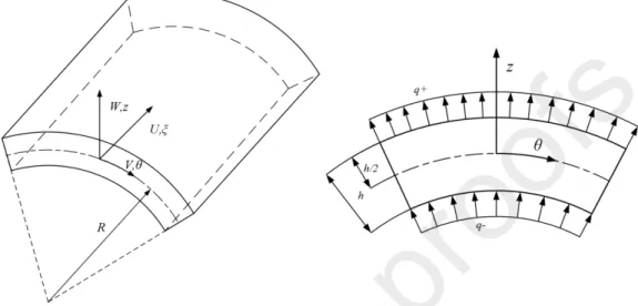
In this paper, we consider an FGM cylindrical shell of length , radius L R and thickness . An orthogonal curvilinear coordinate system , which is shown in Fig. 1, is employed.

h Oz

The neutral surface is assumed to coincide with the middle surface. The displacements of an arbitrary point of the shell in the , and directions are denoted by , and   z u v w ,

(6)

respectively. The Young’s modulus E, Poisson’s ratio  are assumed to be functions of the volume fraction of constituent materials. The shell is subjected to transverse normal loads

and on the outer and inner surfaces, respectively.

 

^,

q^   ^q^

 

^{ }^,

Fig. 1. Geometry and notations of a FGM cylindrical shell 2.1. Displacement fields and strains

The displacement field of the shell in the orthogonal curvilinear coordinate system Ozis expressed by

         

¹

 

(1)

0 0 0

, , , , , , , , , , , ,

! ! !

k k k

K K K

k k k

z z z

u z u v z v w z w

k k k

          ^  

  













where u₀, v₀ and w₀ are the 2D displacements of an arbitrary point in the , and   z directions, respectively. u¹and are the transverse normal rotations corresponding to the , v₁   axes. The other terms in equation (1) are the 2D high-order displacements according to the Taylor series.

The strain–displacements relations given by the linear part of Green-Lagrange strain tensor in the orthogonal curvilinear coordinate system Oz is defined as follows [5]:

(2)

1 1 1 1

, , ,

1 1 1

, , .

z z z

u v v u

R R z w R R z

w v v w u w

R z z R z R z R z

  

 

  

   

  

 

    

           

    

     

      

(7)

Substituting the expressions of the displacement components in equation (1) into equation (2), we obtain the strain field as follows:

- For the displacement model with K 3

 

(3)

2 3 2 3

0 * * 0 * *

2 3 2 3

0 * * 0 * *

2 3

0 * * 0

1 1

, ,

2 3! 2 3!

1 1

2 3! 2 3! ,

1 1

, ,

2 3!

z z z z z z z z

z z z z

z z

R R z

z z z z

z z

R R z

z z

R R

         

        

    



         

        

       



   

            

   

           

 

       

 

2 3

0 * *

1 ,

2 3!

z z z z z

z z

R z^^ ^ z ^ ^ ^

      

- For the displacement model with K2

(4)

2 2

0 * 0 * 0

2 2

0 * 0 *

2 2

0 * 0 *

1 1 1

, , ,

2 2

1 1

2 2 ,

1 1

, ,

2 2

z z

z z z z z z z z

z z

R R z R

z z

R R z

z z

R R z

       

      

       

         

      

       

   

           

   

         

   

          

where

(5)

0 0 1 * 2 * 3 0 0 0

1 2 0

* * 3 0 0

1 2 1

1 2

* 2 * 3 0 0 1 * 2 * 3

0 0

1

, , , , , , ,

, , , , ,

, , , , , ,

z z

z

u u u u v

w w w

v v

v v v

w w

v u u

w Ru

    

    

     



      

    

    

    

     

     

 

    

       

    

 

  

      

    

  

     

     

  



* *

1 2

2 3

0 0 1 * 2 *

1 0 2 3 2 3

, , , 0,

, , , 2 .

z z z

z z z z

w w

Ru Ru

w w w

Rv v Rv Rv v v

  

   

  

 

   

  

 

    

 

  

        

  

2.2. Constitutive relations

The material property gradation of a two-constituent FGM’s in the thickness direction is involved in this study, and the following expression represents the profile of the volume fraction.

(8)

   

^, (6)

FGM t b b

P z  P P V P 

where ¹ ; denotes material parameters, such as the Young’s modulus E and the 2

V z h

 

   P^FGM

Poisson’s ratio  ; and P_t P_b are the parameters at the top and bottom surfaces of the shell, respectively; and is the power-law index that is a positive real number. The FGM material  properties vary smoothly across the shell thickness. Material 1 is placed at the inner surface and material 2 is at the outer surface.

The 3D linear constitutive relations of a cylindrical shell are

(7)

11 12 13

21 22 23

31 32 33

44 55

66

0 0 0

. ,

0 0 0 0 0

z z

C C C

C C

C

 

 

 

 

 

 

 

     

     

     

   

 

   

 

   

 

   

 

     

   

where

, ,

 

  

11 22 33

1

1 1 2

FGM FGM

C C C E 

 

   

  ⁴⁴ ⁵⁵ ⁶⁶ ^{2 1}



^FGMFGM



C C C E

   



  

.

12 21 13 31 23 32

1 1 2

FGM FGM

C C C C C C E 

 

     

 

2.3. Governing equations

The governing equations are based on the equilibrium state and obtained by the use of the principle of virtual displacements. The principle of virtual work in the present case is given as

(8)

 

²

2

1

1 1 0,

2 2

z z z z z z

z

R z d d dz R

h h

q w q w R d d

R R

         



 

             

   

   

 

        

    

        





in which , .

2

0 2 1 8 2

h h

w w w w

 ^      ₀ ₁ ² ₂

2 8

h h

w w w w

 ^     

(9)

Substituting equations (2) – (5) and (7) into equation (8) and integrating this equation through the thickness of the shell we derive:

- For the displacement model with K 3

(9)



⁰ ^* ^* ^* ^* ⁰ ^* ^* ^* ^* ⁰

0 * * * * 0 * *

* * 0 * * 0 * *

z z

z z z z z z

N M N M N M N M Q

S N M N M N M N

M Q S Q Q S Q S

               



             

             

        

       

      

        

       





 

* *

2

0 0 1 1 2 2 0,

z Rd d

p w p w p w R d d

 

 

  

    





  

- For the displacement model with K2

(10)



 ^ ^

0 * * 0 * * 0 0

* * 0 * * 0

0 * * 2

0 0 1 1 0,

z z

z z z

N M N N M N Q N

M N N M N Q S

Q S Q Rd d p w p w R d d

             



             

     

 

       

      

        

       

     



where



^* ^*



^/2 ² ³

/2

, , , 1 1, , , ,

2 6

h

z z z

N M N M z dz

    ^  R



 





   



^* ^*



^/2 ² ³

^ ^ ^{ }

/2

, , , 1, , , , , 1, 1 ,

2 6

h h

z z z

h h

z z z

N M N M z dz Q S z dz

    ^  ^  R

 

   





  



  



^* ^*



^/2 ² ³

/2

, , , 1, , , ,

2 6

h

z z N_ M_ N_ M_ ^ _ z dz



 

  

 





^* ^*



^/2 ² ³ (11)

/2

, , , 1 1, , , ,

2 6

h

z z z

N M N M z dz

    ^  R



 





   



^*



^/2 ²

/2

, , 1, , 1 ,

2

h z h

z z

Q S Q z dz

   ^  R



  





   



^* ^*



^/2 ² ³

/2

, , , 1, , , ,

2 6

h z h

z z Q S Q S_ _ _ _ ^ _ z dz



 

  

 



(10)



^{/ 2}

 

^{/ 2}



1 1 , 0,1, 2.

2 ! 2 !

i i

i

h h

p q q i

R i R i

    

        

   

The equations of equilibrium can be derived from equations (9) and (10) by integrating the displacement gradients by parts and setting the coefficients u_k, v_k and w_k to zero separately.

Thus, one can obtain the equilibrium equations associated with the present quasi-3D type HSDT:

0: N N 0,

u ^ ^

  

 

 

 

0: N N 0,

v ^ ^ Q_

  

   

 

0: Q Q 0 0,

w ^ ^ N_ Rp

  

    

 

1: M M 0,

u ^ ^ RQ_

  

 

  

 

1: M M 0,

v ^ ^ RQ_

  

   

 

1: S S _z 1 0, (12)

w ^ ^ M_ RQ Rp

  

     

 

* *

2: N N 0,

u ^ ^ RS_

  

 

  

 

* *

*

2: N N 0,

v ^ ^ RS_ Q_

  

    

 

* *

*

2: Q Q _z 2 0,

w ^ ^ N_ RS Rp

  

     

 

* *

*

3: M M 0,

u ^ ^ RQ_

  

 

  

 

.

* *

3: M M 2 0

v ^ ^ RQ_ S_

  

    

 

The boundary condition of equation (11) may take one of the following forms:

(11)

- For the boundary condition  const

(13)

0 0 0 0 0 0

1 1 1 1 1 1

* *

* * * *

2 2 2 2 2 2

* *

3 3 3 3

, , ,

, ,

N N u u N N v v Q Q w w

M M u u M M v v S S w w

M M u u M M v v

 

   

     

 

   

 

        

     

- For the boundary condition  const

(14)

0 0 0 0 0 0

0 0 1 1 1 1

* *

* * * *

2 2 2 2 2 2

* *

3 3 3 3

, , ,

, .

M M u u M M v v S S w w

M M u u M M v v

 

   

 

   

 

   

 

        

     

Equations (13) and (14) cover all types of boundary condition, and the number of the boundary conditions equals to the order of the differential equation system.

In the case of a closed cylindrical shell, the boundary condition presented in equation (14) is replaced by a periodic condition with respect to the coordinate. The boundary condition in  equation (13) can be simplified for some common cases as

- For fully clamped boundary condition:

0 1 2 3 0, 0 1 2 3 0, 0 1 2 0, (15)

u  u u u  v    v v v w w w  - For fully simply supported boundary condition:

(16)

* *

0 1 2 3 0 1 2

0, 0, 0.

N_ M_ N_ M_  v  v v v  w w w  - For fully free boundary condition:

* * 0, * * 0, * 0, (17)

N_ M_ N_ M_  N_ M_ N_ M_  Q_ S_ Q_ 

(12)

3. Solving process

3.1. Converting partial differential equations to ordinary differential equations

The equilibrium equation (12) gives us the system of 3K 2 differential equations for displacement components , , and the number of degrees of freedom is

3K2 u_k v_k w_k

Equation (12) is re-written as

 

2 3K2 .

(18)

 

   

2 2 2

1 1 ,11 2 1 ,22 2 2 ,12

0 0

1 3 ,1 0

2 2 2

1 ,12 2 2 ,11 2 2 ,22 2

0 0

1 3 ,2 0

0, 1,..., 1 ,

0, 2 ,..., 2 2

K K

l l l l

i i i i i i

i i

K l

i i

i

K K

k k k k

i i i i i i

i i

K k

i i

i

H H H u H v

H w l K

H u H H H v

H w k K K

   



   



 





 





        

     

 

    



 

        

     

     



 



 



   

2 2

1

1 ,1 3 3 ,11 2 3 ,22 2

0 0

2 ,2 0

,

, 2 3 ,..., 3 2 ,

K K

n n n n

i i i i i i

i i

K n n n

i i q q

i

H u H H H w

H v H q H q n K K

  

 ^ ^



 

 



 

        

    

      



 



herein, the coefficients H are constants, which depend on the radius , the relative thickness R , Poisson's ratio , and Young's modulus of the whole structure. These /

h R _FGM E_FGM

constants are determined by synchronizing the coefficients of the two equations (12) and (18).

We transform partial differential equations (18) into a system of ordinary differential equations. For a closed circular cylindrical shell, we employ an expansion method using trigonometric series with respect to the circumferential variable θ. The periodicity conditions are automatically satisfied. The displacement field and the load are represented by single trigonometric series as follows:

 

0

 

¹

 

²

 

1

, cos sin ,

i i im im

m

u   U  ^ U  m U  m



 

 



  

 

0

 

¹

 

²

 

1

, sin cos ,

i i im im

m

v   V  ^ V  m V  m



 

 



  

(13)

 

0

 

¹

 

²

 

(19)

1

, cos sin ,

j j jm jm

m

w   W  ^ W  m W  m



 

 



  

 

0

 

¹

 

²

 

1

, _m cos _m sin ,

m

q^   Q^  ^ Q^  m Q ^  m



 

 



  

0, 1, ..., , 0, 1, ..., 1.

i K j K

Substituting equation (19) into equation (18) and performing some simple mathematical transformations, we can obtain differential equations to determine Ui0

 

 , Wj0

 

 functions as

(20)

 

   

2 1

0

1 1 ,11 2 0 3 ,1

0 0

1 2 0

1 ,1 3 3 ,11 2 0 0 0

0 0

0, 1,..., 1 ,

, 2 3 ,..., 3 2 .

K K

l l l j

i i i i

i i

K K

n i n n n n

i i i j q q

i i

d dW

H H U H l K

d d

dU d

H H H W H Q H Q n K K

d d

 

  ^ ^



 

  

 

 

    

 

 

 

        

 

 

In the case of symmetrical axial loading, the components V_i0

 

 0.

To determine functions Uim¹

 

 , Vim¹

 

 , Wjm¹

 

 and Uim²

 

 , Vim²

 

 , Wjm²

 

 , we obtain the system of differential equations in the same form as follows:

(21)

 

   

2 2

1 1 ,11 2 1 ,22 2 ,12

0 0

1 3 ,1 0

2 2

1 ,12 2 2 ,11 2 2 ,22

0 0

1 3 ,2 0

1 ,

0, 1,..., 1 ,

0, 2 ,..., 2 2 ,

K K

l l l l

i i i im i im

i i

K l

i im

i

K K

k k k k

i im i i i im

i i

K k

i im

i

d d

H H m H U m H V

d d

H d W l K

d

d d

m H U H H m H V

d d

m H W k K K

H

 



 

 





 





 

   

 

 

   

 

      

 

    

 



 



   

1 2

2

1 3 3 ,11 2 3 ,22

0 0

2 ,2 0

, 2 3 ,..., 3 2 .

K K

n n n n

im i i i im

i i

K n n n

i im q m q m

i

d d

U H H m H W

d d

m H V H Q H Q n K K

 

 



 

 



 

     

 

     

 



In equation (21), we neglect the superscripts 1 and 2 of the quantities Uim

 

 , Vim

 

 and

 

. Wjm 

(14)

3.2. Solving boundary problems by the Laplace transform

The solutions from equations (20) and (21) are obtained using the Laplace transform.

Equation (20) is regarded as a specific case of equation (21) when m0. Here, we study the solution from equation (21).

Let ^U^^im

 

^p , ^V^^im

 

^p và ^W^^jm

 

^p be the image functions of Uim

 

 , Vim

 

 , Wjm

 

 , respectively.

According to the rule of differentiating source functions, we derive:

 

^^im

 

¹⁰^, ²₂

 

²^^im

 

¹⁰ ¹¹^,

im im im im im

d d

U pU p C U p U p pC C

d  d 

 ^ ^  ^ ^ ^

 

^^im

 

²⁰^, ²₂

 

²^^im

 

²⁰ ²¹^, (22)

im im im im im

d d

V pV p C V p V p pC C

d  d 

 ^ ^  ^ ^ ^

 

^^jm

 

³⁰^, ²₂

 

²^^im

 

³⁰ ³¹^.

jm jm jm im im

d d

W pW p C W p W p pC C

d  d 

 ^ ^  ^ ^ ^

where

(23)

     

10 20 30

11 21 31

0 0 0

0 , 0 , 0 ,

, , .

im im im im jm jm

C U C V C W

d d d

C U C V C W

d  _ d  _ d  _

 _  _  _

  

Applying the Laplace transform to equation (21) and using equation (22), we derive the following algebraic equation with respect to ^U^^im

 

^p , ^V^^im

 

^p , ^W^^jm

 

^p :

 

^

^{ }

^

^{ }

^

^{ }

  ^ ^

2 2 1

1 1 ,11 1 ,22 2 ,12 3 ,1

0 0 0

10 11 20 1 30

1 ,11 2 ,12 3 ,1

0 0 0

, 1,..., 1 ,

K K K

l l l l l

im im im

i i i i i

i i i

K K K

l l l

i im im i im i jm

i i i

H H p m H U p m H pV p H pW p

H pC C m H C H C l K



  



  

    

     

  

(24)



   

^

^{ }

^

^{ }

  ^ ^{ } ^

2 2 1

1 ,12 2 2 ,11 2 ,22 3 ,2

0 0 0

10 20 21

1 ,12 2 ,11

0 0

, 2 ,..., 2 2 ,

K K K

k k k k k

im im im

i i i i i

i i i

K K

k k

i im i im im

i i

m H pU p H H p m H V p m H W p

m H C H pC C k K K



  

 

     

      