A systematic presentation of the theory of isothermal surfaces in the context of Möbius geometry can be found in [15]. An extension of the Björling problem to surfaces with constant mean curvature was posed (and solved) in [5]. A natural formulation of the Björling problem in the even more general class of isothermal surfaces reads as follows.
We show that the solution of the discrete Gauss-Codazzi equations with sampled data as an initial condition remains close to the solution of the classical Gauss-Codazzi system for the same. In Section 2 we formulate the Gauss-Codazzi-system for smooth isothermal surfaces in the framework of Cauchy analytical problems and prove the unique local solvability of the Björling problem by the Cauchy-Kowalevskaya theorem. For suitable initial conditions, the convergence of the discrete solutions to the corresponding smooth ones is proved in Section 4.
We begin by summarizing the basic properties of smooth isothermal surfaces and proving our first result on the local solvability of the Björling problem. The following result implies the local solvability of (the restricted version of) the Björling problem for isothermal surfaces, with real analytical data. Such additional constraints are expected to guarantee unique solvability of the Björling problem on the much larger class of isothermal surfaces.
In this section, we give a variant of the definition for discrete isothermal surfaces from [3], which is suitable for passage to the continuum limit.
The Discrete Björling Problem
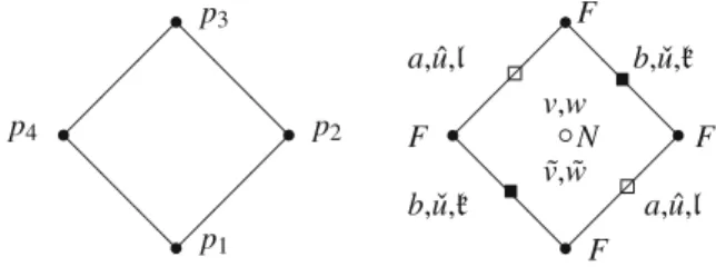
Discrete Quantities and Basic Relations
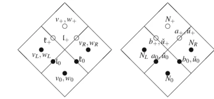
Then use (26) to eliminate sinh2(w) from the first equation and sinh2(v) from the second. Now take the square root and note that v,v˜ have the same sign, and w,w˜ have the same sign according to (25). In particular, we summarize the relations between the geometric quantities (a,b, ˆ . u,uˇ), and of course to Fitself, to the more abstract quantities (v,w,k,l) that satisfy the Gaussian -Codazzi system. (31)–(34).
Discrete Gauss-Codazzi System
Derivation of Equation (31)
Derivation of Equation (32)
More precisely,˜ from (23), one has thatvandwapproximatev˜andw, respectively, to rank˜ 2, in the sense that the family of functions.
Derivation of Equation (33)
4 The Abstract Convergence Result
- Domains
- Statement of the Approximation Result
- Consistency
- Stability
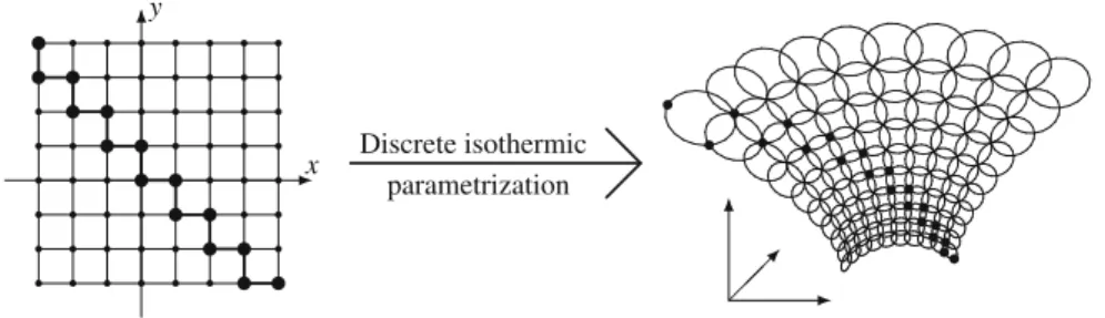
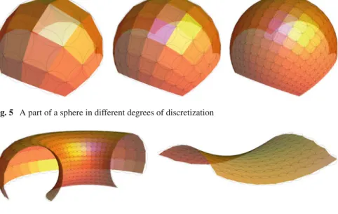
A key concept in the proof is the work with analytic expansions of the quantities v, w, k, and l defined in Section 3.4. In the following, we assume that r >0 and ρ¯>0 are fixed parameters (which will often be omitted in the notations), while h∈(0,ρ)¯ and>0 can vary, with the restriction that A suitable norm to measure the deviation of a discrete solutionθ to a classical solutionθ on the same domainΩρ¯(r|h) is given by the norms of the differences between the four components. Proposition 3 Let an analytic solutionθ to the Gauss-Codazzi system onΩρ¯(r| ¯h) be given, and consider a family(θ)>0 of (a priori not necessarily analytic) solutions θ=(v,w,k, l) for de-discrete Gauss-Codazzi equations onΩ(r|h). Then there are numbers A,B >0and¯>0 such that the following is true for all∈(0,)¯: if θ has sufficient regularity to allow ξ-analytic complex expansions forηnear zero, such that. As it turns out in the proof, the constraint forh is mostly determined by the value of ρ¯. In many examples of interest, ρ¯ is large compared to the area of interest (determined by h¯andr), and consequently, one hash = ¯haabove, that is, convergence occurs on the entire domain of definition ofθ. We begin with an evaluation of the difference between the classical and the discrete Gauss-Codazzi equations. Furthermore, we denote for brevity the difference between the corresponding discrete and continuous quantities byΔ, i.e.Δv= v−vetc. Proof From the analyticity of iθ it is clear that the central difference coefficients obey δξv=∂ξv+gv,ξ, δηv=∂ηv+gv,η etc. Taking the difference between each equation of this system and the corresponding discrete Gaussian equation, Codazzi Equation (31)–(34) gives me. Since the hja are asymptotically analytic on C8, it follows that the modulus hj(Tθ) is uniformly controlled on Ω[x x yy](r|h) by the supremum of the modulus of the components (θ). Second, recalling the definition of · [hx y] and using the Cauchy estimate (42), we obtain for the given ρ∗2k−1 >ρ∗—which remains to be determined—. Fortunately, a close inspection of the terms in (III) reveals, in combination with (57), that we only need bounds on| ˜gj|η,ρ where ρ/ρ¯<1−η∗/h−2/h. Taking the|·|[ηx y∗,ρ]∗ norm on both sides, multiplying byΛ(η∗,ρ∗) <1, and estimating the first few terms as above, we find that. It is straightforward to verify that all the terms on the right-hand side are well defined for the given arguments. Note that the data (v,w,k,l) are ξ-analytic quantities; ironically, one cannot even expect continuity of the respective data fine general. So far, there has been a certain degree of freedom in the choice of f. From now on, there is a unique way to extend the already prescribed f to all Ω(r|2), such that (68) – and incidentally also (67) – applies. We briefly indicate how to proceed in the next step; the further steps are then made inductive in the same way. Then there is a unique choice for f(ξ,η) so that the new vector c= 1. 1) the sin value of the angle between the planes spanned by (a,b) and by (b,c) , equal to tok0(ξ−34), respectively. Continuing this construction in an inductive manner, we enlarge the domain of definition with respect to ξ by 2 in both directions in each step, until f is defined on all Ω(r|2). The verification of (67) is a tedious but straightforward exercise in elementary geometry that we leave to the interested reader. An important point is that the above construction only uses data that can be obtained very directly from the Björling(f,n) data. The maximum-discrete isothermal surface F:Ω(r|h) that is obtained from the fas Björling data—see Proposition 1—is referred to as the increase of (f,n). The plots in Fig. 5 and 6 illustrate that our construction can be used to generate images of the surfaces F with just a few lines of code. Since the quadruple(v,w,k,l) satisfies the discrete Gauss-Codazzi equations, the ξ-analyticity is propagated from the initial strip to the maximal domain of existence, that is, v,w∈ Cω Ω[x y ](r|h). From the estimate (47) it follows in particular that. 70) Here and below we use the slightly ambiguous notationO() to express that the discrete quantities uniformly approximate the associated continuous ones on their respective (real) domainsΩ[x y](r|h)orΩ[x x y](r| h) ,Ω[x yy](r|h), with a maximum error of order. Next, we derive from (70) that also. 71) This indeed follows directly from the definition of these quantities which (71) implies. We only sketch the proof of (71), it is little more than a repeated application of the Gronwall lemma. For further technical details we refer the reader to [2], where the relevant estimations have been performed in a very similar situation, see the proof of Theorem 5.4 therein. Subtract the respective equations, consider (70) and use a standard Gronwall argument to conclude that the validity of (71) extends from the “initial strip” to the entire domainΩ[x x yy](r|h). Due to the uniform proximity of the discrete tangent vectorsδxF,δyF to their continuous counterparts ∂xF,∂yF—. Christoffel Transformation5 The Continuous Limit of Discrete Isothermic Surfaces
From Björling Data to Cauchy Data and Back
Main Result

6 Transformations