Similarly, to construct a feasible interval prediction of 95% in the Gaussian case, we can take x∗0βˆ ± 1.96ˆσ, where ˆσ is the standard error of the regression (also previously denoted as s). Moreover, now that we have introduced “feasible” predictions, we will remain in that world. That is, even if we somehow know the shape of the DGP, we still need to estimate its parameters.
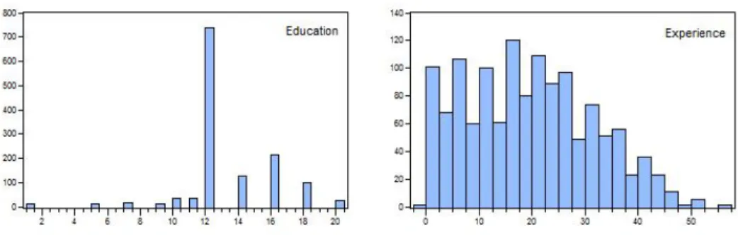
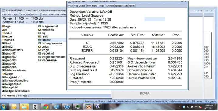
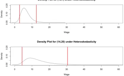
We will illustrate for the Gaussian case without parameter estimation uncertainty, using an approach that closely matches White's test for heteroscedasticity. We will examine the CPS wage data set, which contains data on a large cross-section of individuals on wages, education, experience, gender, race, and union status. However, since we believe in the parsimony principle, we will limit ourselves to a linear model in the absence of overwhelming evidence in favor of a non-linear model.
Using simulation, simply construct the density prediction of the object of interest (eg, W AGE rather than nW AGE) whose sample mean across simulations is consistent with the conditional population mean. However, in more complex environments, we will need to obtain the CI directly from the simulated data, so we will do this here by sorting the sample plots and taking the left and right endpoints to be the values 0.025% and 0.975% . respectively. So even with log homoscedasticity, the variance of the y level will depend on x.
A quick way to think about the algorithm in the previous section is the following: Since residuals are Gaussian, y is Gaussian. We will now accurately estimate the first term and include it in our density prediction. In this environment we will find the distinction to be of little numerical significance, but for other datasets it will be of dramatic importance.
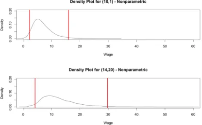
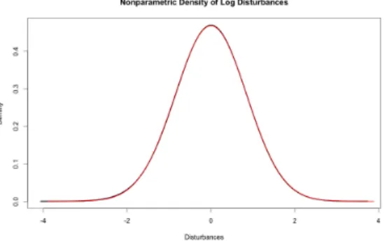
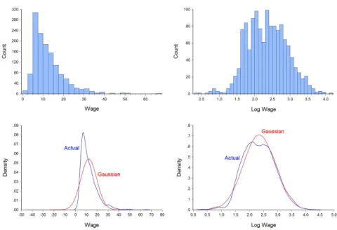
In this section, we will make density predictions for our dataset, dropping the assumption that perturbations are Gaussian. For now, we will assume that we can estimate parameters without uncertainty and that disturbances are homoscedastic. The first thing we will note is that density predictions under the assumption of Gaussian perturbations will generally perform quite poorly because the perturbations of the level model are clearly non-Gaussian.
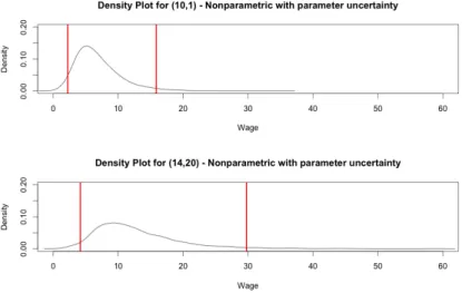
Therefore, we move to a nonparametric prediction of the density, including the parameter uncertainty - although as before we will find that non-parameter.
Non-Parametric Estimation of Conditional Mean Functions
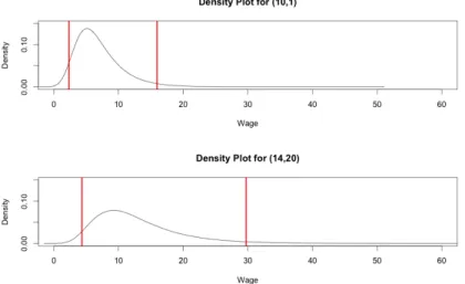
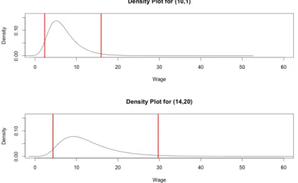
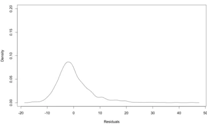
Here, parameter uncertainty in the wage density is taken into account, and the density of residuals is now estimated non-parametrically. The model is directly in salary. The top graph is estimated wage density with 10 years of education, 1 year of experience. One can also mix Taylor and Fourier approximations by going back not only on powers and cross products ("Taylor expressions") but also on various sines and cosines ("Fourier expressions").
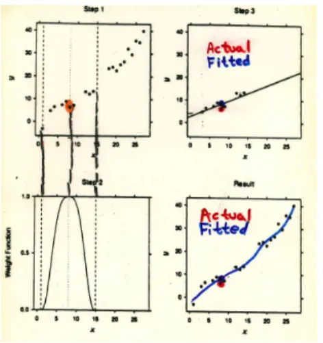
In principle, of course, an infinite number of series terms is required, but in practice nonlinearity is often quite mild, so that only a few series terms are required (e.g. quadratic). 5Note that a product of dummies is one if and only if both individual dummies are one. If we want to predict y for an arbitrary x∗, it is natural to examine and average the y's that occurred for close x's.
That is, we use a bi-squared robustness weight, whereby larger observations with larger absolute residuals at iteration (0) are progressively downgraded further, and observations with absolute residuals greater than six times the median absolute residual are completely eliminated. Economic time series data tend to trend, so x∗ may often be outside the observed x. This can create serious problems for local levelers, as there may not be any nearby "nearest neighbors", for example.
Polynomial and Fourier global smoothers, on the other hand, can be easily extrapolated to short-horizon out-of-sample forecasts. If we want to know what y is likely to go with x∗, an obvious strategy is to look at the y's that went with x's nearest x∗. And the NN idea can be used to not only produce point forecasts (eg by fitting a constant to the y's), but also to produce density forecasts (by fitting a distribution to the y's).
Wage Prediction, Continued
Exercises, Problems and Complements
Now consider the operating point prediction for y given that x = x∗, ˆy = ˆβx∗, and consider the variance of the corresponding prediction error. In this expression, the first term accounts for the normal perturbation uncertainty, and the second term accounts for the parameter estimation uncertainty. Together, the results suggest an operating density prediction that takes parameter uncertainty into account.
Note that when parameter uncertainty exists, the closer x∗ is to meanx(0), the smaller the prediction-error variance. The ideas sketched here can be shown to carry over to more complicated situations (eg, non-Gaussian, y and x do not necessarily have zero mean, more than one regressor, etc.); it remains true that the closer x is to its mean, the narrower the prediction interval. In cross-sections, all forecasting has an “in-sample” flavor insofar as the X∗ for which we want to forecast y is usually within the historical X .
So far we have emphasized perturbation uncertainty and parameter estimation uncertainty (which is partly due to data uncertainty, which again has several components). All our models are deliberate simplifications, and the fact is that different models produce different predictions. Somehow we need to regain degrees of freedom, so dimensionality reduction is key, leading to ideas of variable selection and "sparseness", or shrinkage and "regularization".
Neural networks constitute a special non-linear functional form associated with repeated linear combinations of inputs through non-linear "clamping" functions. We speak, for example, of a "one-output forward neural network with n inputs and 1 hidden layer with q neurons". Unattractive in that the fit at the end is affected by the data at the beginning (for example).
A linear spline is therefore piecewise linear, continuous but not differentiable at the nodes. This adds constraints (two at each end), restoring the degrees of freedom and thus allowing more knots. You'd like to have more nodes in the rough areas of the function being estimated, but of course you don't know where those areas are, so that's tricky.
Notes