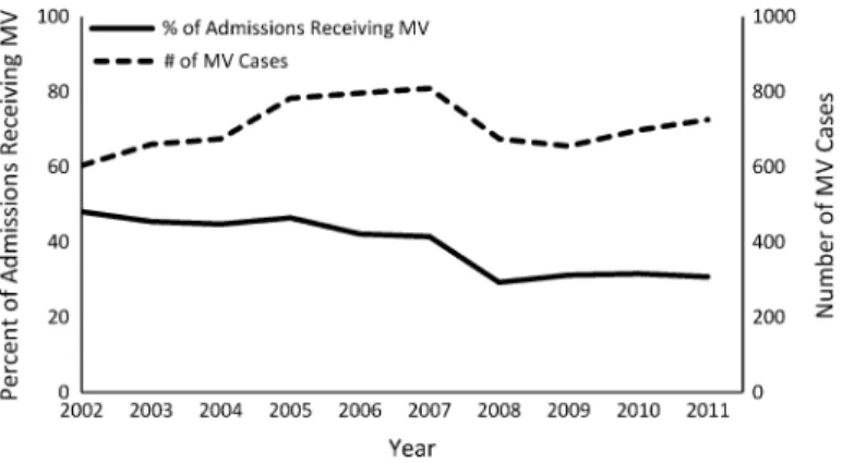
Analyzes for trends in tidal volume change over time included a dependent (outcome) variable of tidal volume and an independent variable (exposure) of time (year of intensive care unit admission). We identified 7083 patients receiving invasive mechanical ventilation in the MICU and 3085 patients in the CCU between 2002 and 2011.
Introduction
The instrument must be correlated with the treatment and explain a significant part of the variation in the treatment: The less variation in the treatment that the instrument explains (the “weaker” the instrument is), the greater the variance of the obtained estimates. The instrument must be independent of the outcome through any mechanism other than the treatment: This remains one of the major challenges in accurately applying IVAs to medical data, as it is difficult to identify instruments that have no correlation with any unobservable clinical variation beyond treatment.
Methods .1 Dataset
Methodology
It is impossible for all the people in the dormitory to be discharged before any of the people who are not in the dormitory. In addition to controlling for thewest_initial_team_census, we also controlled for the total number of boarders under the care of the MICU team.

Pre-processing
The linear assumptions of the Cox models are strong and not justified a priori, therefore to test for potential non-linearities in the instrumental model we used the Vuong and Clarke tests from the SemiParBIVProbitpackage. Finally, a count of the total number of patients treated by the MICU team is generated and added to each row ofdf5.
Results
In the resulting table, rows pertaining to the population of interest (ie, medical patients who incurred an MICU stay at some point during their hospitalization) will have data corresponding to both the left (transfers) and right (med_service_only) tables. We identified a number of cases in the dataset where death occurred within minutes or hours of discharge from the ICU.
Next Steps
That is, the effect they estimate is the local effect on the patients whose treatment is affected by the instrument. This is called the Local Average Treatment Effect (LATE) and is estimated by an IVA if there is heterogeneity in the treatment effects.
Conclusions
Mortality Prediction in the ICU Based on MIMIC-II Results from the Super ICU Learner Algorithm (SICULA) Project. In this chapter, we illustrate the use of MIMIC II clinical data, non-parametric prediction algorithm, ensemble machine learning and the Super-learner algorithm.
Introduction
Given the complexity of the processes underlying death in intensive care patients, this assumption may be unrealistic. Given that the true relationship between ICU mortality risk and explanatory variables is unknown, we expect that prediction can be improved by using an automated nonparametric algorithm to estimate the risk of death without requiring any specification about the form of the underlying relationship.
Dataset and Pre-preprocessing
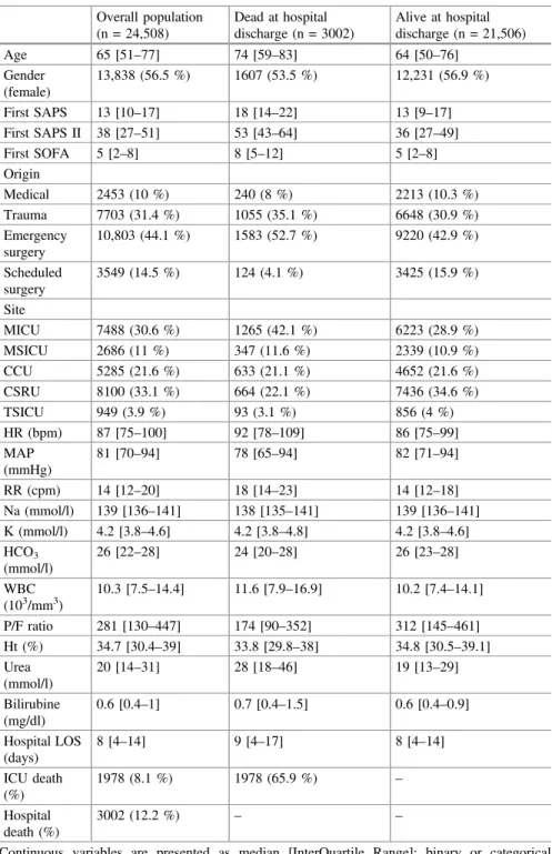
Data Collection and Patients Characteristics
Patient Inclusion and Measures
Methods
Prediction Algorithms
This algorithm was included in the SL library so that revised fits of the SAPS II score based on the current data were also competed against other algorithms. The data used in our prediction algorithm included the 17 variables used in the SAPS II score: 13 physiological variables (age, Glasgow coma scale, systolic blood pressure, heart rate, body temperature, PaO2/FiO2 ratio, urinary output, serum urea nitrogen level, white blood cell count, serum bicarbonate level, sodium level, potassium level and bilirubin level), type of admission (scheduled surgical, unscheduled surgical or medical), and three underlying disease variables (acquired immunodeficiency syndrome, metastatic cancer and hematological malignancy derived from ICD-9 discharge codes).
Performance Metrics
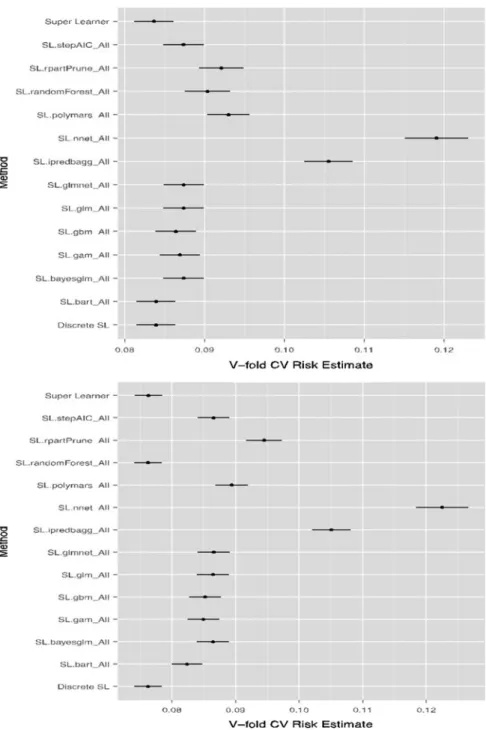
Performance measures are aggregated over all 10 iterations, providing a cross-validated estimate of the mean squared error (CV-MSE) for each algorithm. Subsequently, the prediction rule consisting of the CV-MSE-minimizing weighted convex combination of all candidate algorithms was also calculated and rebuilt on all data.
Analysis
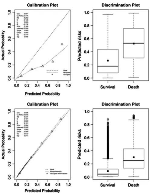
- Discrimination
- Calibration
- Super Learner Library
- Reclassification Tables
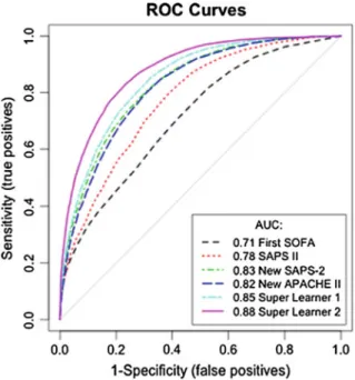
Compared to the classification provided by the original SAPS II, the updated SAPS II, or the revised APACHE II score, the results based on the Super Learner resulted in the downgrading of the vast majority of patients to a lower risk stratum. We calculated the cNRI and IDI considering each Super Learner proposal (grade A) as the updated model and the original SAPS II scores, the new SAPS II and the new APACHE II scores (grade B) as the starting model.
Discussion
Compared to the new SAPS II or the new APACHE II score, both Super Learner proposals resulted in a reclassification of a large proportion of patients, especially from high predicted probability strata to lower strata.
What Are the Next Steps?
Conclusions
Clermont G, Angus DC, DiRusso SM, Griffin M, Linde-Zwirble WT (2001) Predicting in-hospital mortality for intensive care unit patients: a comparison of artificial neural networks with logistic regression models. Kim S, Kim W, Park RW (2011) A comparison of mortality prediction models in the intensive care unit using data mining techniques.
Introduction
Perhaps even more noteworthy is the use of ICU mortality prediction in the fields of health research and administration, which often involve examining cohorts of critically ill patients. Traditionally, such population-level studies have been more widely accepted as applications of mortality prediction based on cohort derivation of prediction models.
Study Dataset
In intensive care, a number of SOI (disease severity) scores have been introduced to predict outcomes, including death. However, for the vast majority of ICU admissions in MIMIC-II, measurements of these common clinical variables were obtained at the beginning of the ICU admission, or at most within the first 24 hours.
Pre-processing
In MIMIC-II, this binary outcome variable can be obtained by comparing the date of death (found in the d_patientstable table) and the date of hospital discharge (found in the theicustay_detailtable). If we were to focus on a longer period of time until death after discharge, we would extract the date of mortality to try to predict survival time.
Methods
Analysis
Visualization
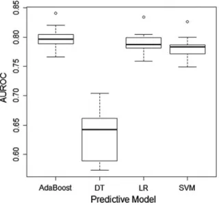
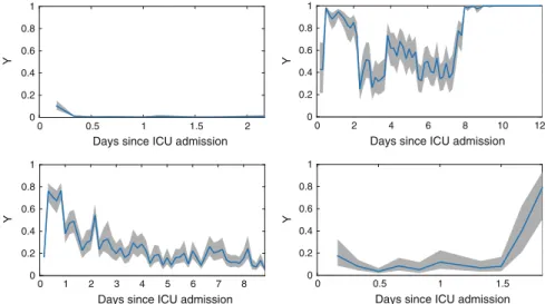
This is most likely due to the fact that the mortality rate is much lower among younger patients than older patients, and predictive models can achieve high accuracy by biasing to predict low mortality risks (however, this will result in low sensitivity ). Therefore, it is important to note that although Fig.21.2 conveys a sense of overall accuracy, it does not reveal sensitivity, specificity, positive predictive value or negative predictive value.
Conclusions
Next Steps
Since the machine learning models discussed in this chapter were purely empirical, the explicit addition of clinical expertise through the Bayesian paradigm may improve predictive performance. Finally, data quality is often overlooked but plays an important role in determining what predictive performance is possible with a given set of data.
Connections
Bayesian methods strike a balance between subject matter expertise (for predicting ICU mortality, this would correspond to clinical expertise regarding mortality risk) and empirical evidence in clinical data. Images or other third-party material in this chapter are included in the work's Creative Commons license, unless otherwise indicated in the credit line; if such material is not included in the Creative Commons license of the work and the corresponding action is not permitted by legal regulations, users will need to obtain permission from the license holder to copy, adapt or reproduce the material.
Introduction
Accordingly, algorithms have been proposed in the literature that improve performance by using data fusion techniques to combine vital signs with other parameters such as biochemistry and demographic data [18,19] . The remainder of this chapter is designed to equip the reader with the necessary tools to develop and evaluate data fusion algorithms for prediction of clinical deterioration.
Study Dataset
EWSs are aggregated scores calculated from a set of routinely and frequently measured physiological parameters known as vital signs. However, there is room to improve their performance as most EWSs use simple formulas that can be calculated manually at the bedside, and take only a limited number of vital signs as input [17].
Pre-processing
Non-invasive measurements were replaced with surrogate invasive values by correcting for the observed deviations between the two measurement techniques when both were used in the same four-hour periods (the median differences between invasive and non-invasive measurements were 2, 7 and 6 mmHg for systolic, diastolic and mean blood pressure respectively). Finally, the dataset contained missing values where parameters were not measured within certain four-hour periods.
Methods
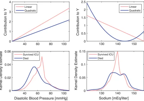
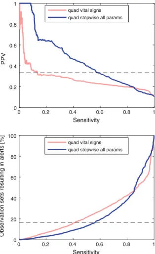
The importance of choosing the relationship between the predictor variables and the estimate is demonstrated in Figure 22.1. Third, stepwise regression was used to avoid including terms that would not improve model performance.
Analysis
The quadratic algorithm using only vital signs has a much lower sensitivity of 13.2 % than the equivalent algorithm using stepwise inclusion of all parameters, at 59.3 % when the PPV criterion is met. Similarly, when using the alarm rate criterion, the sensitivity of the vital signs algorithm is 41.4%, also lower than that of the algorithm using stepwise inclusion of all parameters, at 56.3.
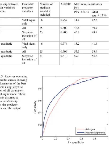
Discussion
Inclusion of additional physiological parameters beyond vital signs alone resulted in improvements in algorithm performance in this study when evaluated using AUROC, as previously observed [18,19], and when evaluated using minimum sensitivities corresponding to the requirements clinical. In this case study we presented AUROC and maximum sensitivities when the algorithms were constrained to a minimally acceptable PPV and a maximally acceptable alarm rate [ 23 ].
Conclusions
Further Work
Personalised Prediction of Deteriorations
Buist MD et al (1999) Recognition of clinical instability in hospitalized patients before cardiac arrest or unplanned intensive care admission. Saeed M et al (2011) Multiparameter intelligent monitoring in intensive care II: a publicly available intensive care unit database.
Incentives for Using Propensity Score Analysis
Understand the incentives and drawbacks of using propensity score analysis for statistical modeling and causal inference in EHR-based research. Appreciate concepts underlying propensity score analysis with EHRs, including stratification, matching, and inverse probability weighting (including straight weighting, stabilized weighting, and doubly robust weighted regression).
Concerns for Using Propensity Score
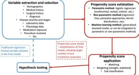
Although large-scale EHRs often have sample sizes large enough to allow high-dimensional investigation, dimension reduction is still useful for the following reasons: (i) to simplify the final model and make interpretation easier, (ii) to enable sensitivity analyzes to create research higher order terms or interaction terms for those covariates that may have a correlation or interaction with the outcome, and (iii) depending on the research question, the study cohort may still be small despite being from a large database, and dimension reduction is therefore crucial for a model to be valid.
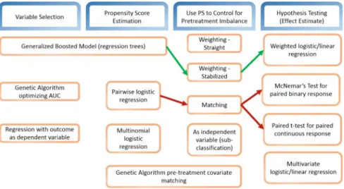
Different Approaches for Estimating Propensity Scores
It is possible to use a nonparametric model to estimate the propensity score [13], such as regression trees, piecewise approaches, and kernel distributions. For example, some studies use a genetic algorithm to select variables and model specifications for a conventional logistic regression to estimate the propensity score [ 15 ].
Using Propensity Score to Adjust for Pre-treatment Conditions
In EHR data research, we have access to a large number of pretreatment covariates that we can extract from the database and use in the propensity score model. Propensity score analysis is a powerful tool to simplify the final model, while a large number of pretreatment conditions can be included.
Study Pre-processing
A major criterion for determining the effectiveness of a pharmacologic agent in controlling Afib with RVR is the time to completion of the RVR episode. The first step is to estimate the propensity score (probability of being assigned to a treatment group given pre-treatment covariates).
Study Analysis
Study Results
Conclusions
Next Steps
Patorno E et al (2014) Studies with many covariates and few outcomes: selection of covariates and implementation of propensity score-based confounding adjustments. Feng P et al (2012) Generalized propensity score for estimating the mean treatment effect of multiple treatments.
Introduction
Understand how Markov models can be used to analyze medical decisions and perform cost-effectiveness analyses. The last part discusses a practical example, inspired by the medical literature, in which a Markov chain will be used to perform the cost-effectiveness analysis of a given medical intervention.
Formalization of Common Markov Models
- The Markov Chain
- Exploring Markov Chains with Monte Carlo Simulations
- Markov Decision Process and Hidden Markov Models
- Medical Applications of Markov Models
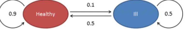
Using the example shown in Fig.24.1, we will estimate the probability that someone is healthy or sick in 5 days, knowing that he is healthy today. In the medical literature, Markov models have explored very different problems such as the timing of liver transplantation [8], HIV therapy [9], breast cancer [10], Hepatitis C [11], statin therapy [12] or treatment of hospital discharge [5,13 ].
Basics of Health Economics
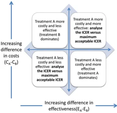
The Goal of Health Economics: Maximizing Cost-Effectiveness
Controlled Markov models can be solved using algorithms such as dynamic programming or reinforcement learning, which aim to identify or approximate the optimal policy (set of rules that maximizes the expected sum of discounted rewards). Markov models can be used to describe different health states in a population of interest and to detect the effects of different policy or therapeutic choices.
De fi nitions
The analysis will calculate the relative costs of improving health and provide metrics to optimally inform decision makers. Schematically, this means that if the ICER of a new medical intervention is below a certain threshold, health benefits can be achieved with an acceptable level of expenditure.
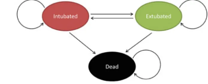
Case Study: Monte Carlo Simulations of a Markov Chain for Daily Sedation Holds in Intensive Care,
By simulating the distribution of the average number of ventilator-free days and its characteristics can be calculated for both strategies (functionMCMC_solver.m). It belongs to the upper right quadrant of the CE plane, Table 24.9 Calculation of the number of ventilator-free days by Monte Carlo (10,000 simulated cases).
Model Validation and Sensitivity Analysis for Cost-Effectiveness Analysis
Some medical interventions may or may not be funded depending on the model's assumptions. In addition to validating the Markov model used to simulate the states and transitions for the system of interest, it is also important to perform a sensitivity analysis on the assumptions and parameters used in the simulation.
Conclusion
For example, the authors report a 28-day mortality rate of 29 and 35% in the intervention and control groups, respectively. The theoretical concepts introduced in the opening paragraphs of this chapter were applied to a concrete example from the medical literature.
Next Steps
Schaefer AJ, Bailey MD, Shechter SM, Roberts MS (2005) Modeling medical treatment using Markov decision processes. Alagoz O, Maillart LM, Schaefer AJ, Roberts MS (2004) The optimal timing of living donor liver transplantation.
Introduction
Blood Pressure and the Risk of Acute Kidney Injury in the ICU: Case-Control Versus Case-Crossover Designs. Introduce two different approaches, a case-control and a case-crossover design, to study the effect of transient exposure of hypotension on the risk of acute kidney injury (AKI) development in intensive care unit (ICU) patients.
Methods
Data Pre-processing
A Case-Control Study
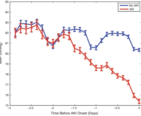
Note that the mean arterial pressure of the AKI group differed from that of the controls before the onset of AKI. The mean arterial blood pressure of the AKI group changed from that of the controls during the second day before the onset of AKI, and both groups showed significant diurnal changes.
A Case-Crossover Design
The minimum MAP from a 3-hour control period during the first 12 hours in the ICU, when the same patient's renal function was still normal, was used as the exposure for the controls. In addition, time-varying confounding factors (mechanical ventilator, vasopressors, temperature, heart rate, white blood cell count, SpO2) were included in the multivariate conditional logistic regression model.
Discussion
Conclusions
Lehman LH, Saeed M, Moody G, Mark R (2010) Hypotension as a risk factor for acute kidney injury in ICU patients. Lehman LH, Saeed M, Talmor D, Mark RG, Malhotra A (2013) Methods of blood pressure measurement in the ICU.
Introduction
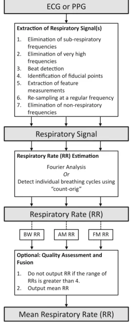
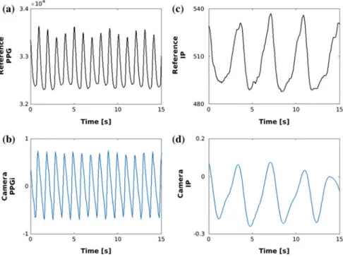
Many algorithms have been developed to estimate RR from ECG and PPG [10,12], but they have not yet been widely adopted in clinical practice. In this case study, we demonstrated the use of exemplary techniques for ECG and PPG.
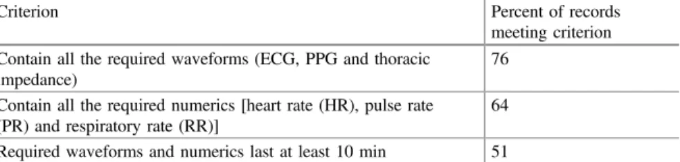
Study Dataset
This ensured that any gaps in the data due to changes in patient monitoring or data collection errors were retained in the analysis. Inspection of the data set revealed a significant difference in the distribution of IP RR measurements acquired from neonatal and adult patients, as illustrated in Fig.26.2.
Pre-processing
Count-orig involves normalizing the signal, identifying pairs of maxima that exceed a threshold value, and identifying reliable breaths as signal periods between pairs of maxima that contain only one minimum below zero.
Methods
The first step of Smart Fusion is to assess the quality of the RR estimates derived from the three modulations. If all three estimates are within 4 bpm of each other, then the final RR estimate is generated as the average of the estimates.
Results
An additional quality assessment and fusion rate, the “Smart Fusion” method [19], was optionally performed in an attempt to increase the accuracy of the RR estimates. Consequently, only 6% of ECG data and 7% of PPG data were included in the analysis.
Discussion
Conclusions
Further Work
Non-contact Vital Sign Estimation
During the period the patient had a heart rate of 60 beats/min and a respiratory rate of 15 breaths per minute (bpm). Meredith DJ, Clifton D, Charlton P, Brooks J, Pugh CW, Tarassenko L (2012) Photoplethysmographic derivation of respiratory rate: a review of relevant physiology.
Introduction
Furthermore, alarm thresholds are often adjusted in an ad hoc manner, based on how bothersome the alarm is perceived by the attending clinical team. The alarm is triggered by loud noise manifesting as high-amplitude (±2 mV) oscillations on the ECG at approximately 5 Hz, starting a little more than halfway through the snapshot (and a little less than 10 s from the vertical VT marker ).
Study Dataset
A promising solution to the false alarm issue comes from multiple variable data fusion, such as HR estimation by fusing the information from synchronous ECG, ABP and photoplethysmogram (PPG) from which oxygen saturation is derived [18]. 22] and Li and Clifford [23] suppressed false ECG alarms by assessing the signal quality of ECG, ABP and PPG.
Study Pre-processing
The DTW-based SQI resampled each beat to match the ongoing beat template, so it was derived using DTW. PPG SQI measurements included DTW-based SQI [ 32 ] and the first two parameters of Hjorth [ 20 ], which estimated the dominant frequency and half-bandwidth of the PPG spectral distribution.
Study Methods
The predicted output of the likelihood function (L) from the forest is the inverse log of the sum of the contribution of each tree plus the intercept term (27.1). The predicted likelihood of the prior forest (Li) and the likelihood of the forest with the two updated trees (Li+1) were calculated.
Study Analysis
In the algorithm validation phase, the classification performance of the algorithm was evaluated using 10-fold cross-validation. Then, nine folds were used for model training and the last fold was used for validation.
Study Visualizations
This process was repeated ten times as one integral procedure, with each of the folds used exactly once as the validation data. The result of 10-fold cross-validation with different options of operating points is shown in Table 27.2.
Study Conclusions
Second, medical history, demographics and other medical data were not available and therefore used to adjust thresholds. Finally, information regarding repeated alarms was not used to dynamically adjust false alarm suppression based on earlier alarm frequency during the same ICU stay.
Next Steps/Potential Follow-Up Studies
Chambrin MC (2001) Review: alarms in the intensive care unit: how to reduce false alarms. Li Q, Clifford GD (2012) Signal quality and data fusion for false alarm reduction in the intensive care unit.
Introduction
To compare and evaluate the performance of the structured data extraction method and the natural language processing (NLP) method in identifying patient cohorts using the Medical Information Mart for Intensive Care (MIMIC-III) database. To evaluate the performance of the structured data extraction method and the NLP method when used for patient cohort identification.
Methods
- Study Dataset and Pre-processing
- Structured Data Extraction from MIMIC-III Tables
- Unstructured Data Extraction from Clinical Notes
- Analysis
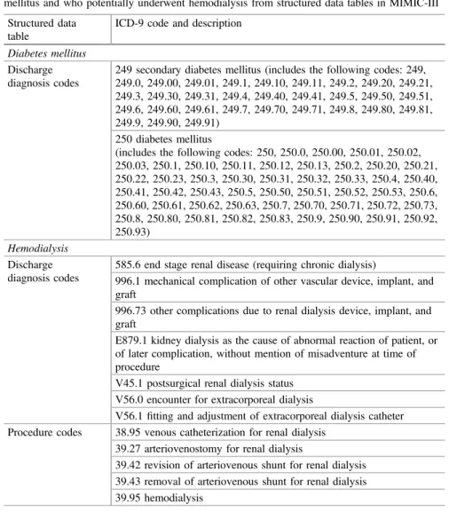
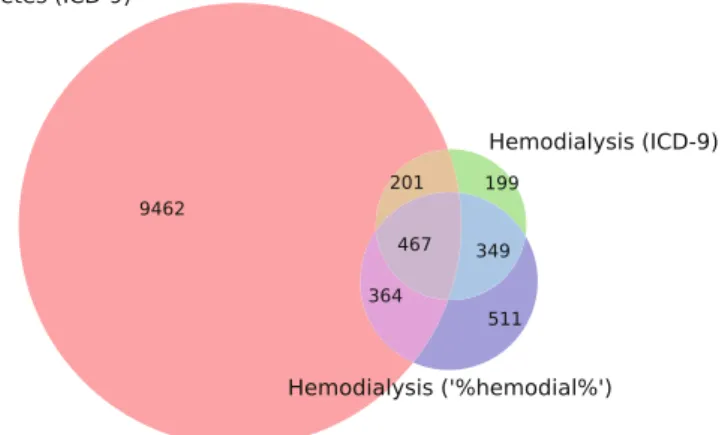
Therefore, in this case study we sought to determine whether using NLP on the unstructured clinical notes of this population would help improve structured data extraction. To identify diabetes mellitus patients who underwent hemodialysis during their intensive care unit stay, we scanned the clinical notes containing the terms “diabetes mellitus” and “hemodialysis”.
Results
We used this validation database to evaluate the precision and recall of both the structured data extraction method and the clinical NLP method. We also analyzed the clinical notes of the 19 patients identified as FP using the structured data extraction method.
Discussion
Conclusions
Segal JB, Powe NR (2004) Accuracy of identification of patients with immune thrombocytopenic purpura by administrative records: a data validation study. Abhyankar S, Demner-Fushman D, Callaghan FM, McDonald CJ (2014) Combining structured and unstructured data to identify a cohort of ICU patients receiving dialysis.
Introduction
Patients with sepsis are at high risk for mortality (approx. and the ability to predict outcomes is of great clinical interest. We show that using hyperparameter selection methods, MSE can predict patient outcome more accurately than APACHE score.
Study Dataset
The APACHE score [2] is widely used to predict mortality, but has significant limitations in terms of clinical application, as it often fails to accurately predict individual patient outcomes and does not take into account dynamic physiological measurements.
Study Methods
Each time a new AUROC is calculated, the MSE parameter set as well as the AUROC is added to the ytest toxtestand. By iterating through this process, new sets of MSE parameters yield higher and higher AUROCs.

Study Analysis
Study Visualizations
Study Conclusions
Discussion
Finally, a more thorough comparison between hyperparameter selection techniques will help understand why a given hyperparameter selection technique performs better than others for a particular prediction problem. In particular, the hyperparameter selection techniques also have parameters, and a better understanding of the impact of these parameters on the results requires further investigation.
Conclusions
Hemberg E, Veeramachaneni K, Dernoncourt F, Wagy M, O'Reilly U-M (2013) Effective use of training sets for blood pressure prediction in a large-scale learning classifier system. Hemberg E, Veeramachaneni K, Dernoncourt F, Wagy M, O'Reilly U-M (2013) Imprecise selection and skill approximation in a large-scale evolutionary rule-based system for blood pressure prediction.
![Untitled - Artikel Universitas Bandar Lampung [UBL]](data:image/gif;base64,R0lGODlhAQABAIAAAP///wAAACH5BAEAAAAALAAAAAABAAEAAAICRAEAOw==)