ANALYSING POTATO PRICE VOLATILITY IN SOUTH AFRICA BY
Moabelo Julith Tsebisi
A MINI-DISSERTATION submitted in partial fulfilment of the requirements for the degree
of
Master of Science in Agriculture in
Agricultural Economics in the
Faculty of Science and Agriculture
(School of Agriculture and Environmental Sciences) at the
UNIVERSITY OF LIMPOPO, SOUTH AFRICA
SUPERVISOR: MRS CL MUCHOPA CO-SUPERVISOR: PROF A BELETE
2019
i DECLARATION
I, Moabelo Julith Tsebisi, declare that the research report entitled: ANALYSING POTATO PRICE VOLATILITY IN SOUTH AFRICA: submitted to the University of Limpopo in partial fulfilments for the requirement of the degree of Master of Science in Agricultural Economics, has not been submitted before and that all sources or materials used have been duly acknowledged.
Student: ……… date:……….
Ms Moabelo JT
ii DEDICATION
I wish to dedicate this paper to my departed fiancé, Lungelo Andries who believed so much in me and my education unfortunately Almighty has called him in the first year of my master’s studies and would not see much of my success.
iii ACKNOWLEDGEMENT
I firstly thank the master of all creation (Almighty) for his abundant grace. If it was not of him, I could not have been where I am today. Special thanks go to my supervisor Mrs CL Muchopa and Co-supervisor Prof A Belete for their words of encouragement and support.
I extend my sincere appreciation to Laryssa van der Merwe from Potato South Africa (PSA) who provided me with all the data needed in this dissertation pertaining to potatoes.
To my parents Moabelo Lesiba and Moabelo Raisibe thank you for your support. Mme Motswadi you have been a pillar of my strength, thank you for supporting me in every way, it is true when they say Mmago ngwana o swara thipa ka bogaleng. My children Katlego and Unako, you have been my inspiration. My siblings, Lusty, Lamenta, Monica, Phillipine and Mawina Moabelo, thank you all for your support.
iv ABSTRACT
Potato is perceived as an excellent crop in the fight against hunger and poverty. The recent high potato price in South Africa has pushed the vegetable out of reach of the poorest of the poor. The study attempts to analyse potato price volatility in South Africa and furthermore assess how various factors were responsible for the recent potato price volatility. Quarterly data for potato price, number of hectares planted, rainfall and temperature levels from 2006q1 to 2017q4 was collected from various sources and were used for analysis. The total observation of 48.
The volatility in the series was determined by performing ARCH/GARCH model. GARCH model indicates an evidence of GARCH effect in the series, meaning that GARCH model influences potato price volatility in South Africa. The Johansen cointegration used both trace and eigenvalue to test the existence of a long run relationship between potato price and various variables. The cointegration results were positive indicating that there exists long run relationship amongst variables. The study further used Johansen cointegration as well as standard error to determine the number of cointegrating variables in the long run. The results indicated that the number of hectares planted and rainfall level have significant relationship with potato price. Wald tests was used to check whether the past values of number of hectares planted and rainfall level influenced the current value of potato price. The Walt test results concluded that there is no evidence of short run causality running from number of hectares planted and rainfall level to potato price. In the study, ECM model was used to forecast the potato price fluctuation in South Africa.
The study recommends that farmers need to engage in contract market so as to minimize the risk of potato price volatility. The Department of Agriculture should forecast agricultural commodities price volatility and make information accessible to the farmers so that they are able to adopt strategies that will assist them to overcome crisis.
Keywords: Potato price, GARCH model, VECM, Volatilities, ECM model, Forecasting
v TABLE OF CONTENTS
DECLARATION ... i
DEDICATION ...ii
ACKNOWLEDGEMENT ... iii
ABSTRACT. ...iv
LIST OF TABLES ... vii
LIST OF FIGURES ...ix
LIST OF ACRONYMS ... x
CHAPTER ONE: INTRODUCTION. ... 1
1.1 Background ... 1
1.2 Problem statement ... 3
1.3.Motivation ... 4
1.4 Aim of the study ... 4
1.5 Study objectives ... 4
1.6 Hypotheses ... 4
CHAPTER TWO: LITERATURE REVIEW ... 4
2.1 Introduction ... 5
2.2 Defining price volatility and volatility ... 5
2.3 Factors affecting potato price volatility ... 6
2.3.1 Weather condition. ... 6
2.3.2 Market factors ... 7
2.3.3 Production cost ... 9
CHAPTER THREE: RESEARCH METHODOLOGY ... 11
3.1 Introduction ... 11
3.2 Potato production regions ... 11
3.3. Data collected and source of data ... 13
3.4 Method of analysis ... 14
3.4.2Measure to evaluate volatility . ... 14
3.4.2.1 Modeling volatility ... 15
vi
3.4.2.2 The (ARCH) Autoregressive Conditional Heteroskedasticity Model ... 15
3.4.2.3 The (GARCH) General Autoregressive Conditional Heteroskedasticity Model ... 16
3.4.2.4 Diagnostic check ... 17
3.4.3 Unit roots tests ... 17
3.4.3.1 Testing for cointegration ... 18
3.4.3.2 VECM ... 19
3.4.3.3 Diagnostic check ... 20
3.5 Forecasting with ECM model ... 20
3.5.1 Forecasting accuracy ... 20
3.6 Analysis of objectives ... 21
CHAPTER FOUR: RESULTS AND DISCUSSION. ... 22
4.1 Introduction ... 22
4.2.1 Measuring to evaluate volatility ... 25
4.2.2 Testing for clustering volatility ... 23
4.2.3 Testing for ARCH effect ... 24
4.2.4 Testing GARCH effect... 25
4.2.5 Diagnostic check ... 26
4.2.5.1 ARCH effect test ... 26
4.2.5.2 Serial correlation ... 26
4.3 Testing for stationarity ... 28
4.3.1 Unit root test ... 25
4.3.2 VAR Lag Order Selection ... 29
4.3.3 Johansen test for cointegration ... 30
4.3.3.1 Unrestricted cointegration rank test (Trace) ... 31
4.3.3.2 Unrestricted cointegration rank test (Maximum Eigenvalue) ... 31
4.3.3.3 Long run cointegration ... 32
4.3. VECM... 34
4.3.1 Short run causality ... 34
4.3.5 Testing for serial correlation ... 35
4.4 Forecasting ... 36
vii CHAPTER FIVE: SUMMARY, CONCLUSION AND POLICY RECOMMENDATIONS. 40
5.1. Introduction ... 40
5.2 Summary ... 40
5.3 Conclusion ... 41
5.3 Recommendation ... 41
REFERENCES ... 43
viii LIST OF TABLES
Table 1: Data collection and sources of data. ... 13
Table 2: Method of analysis. ... 21
Table 3. Coefficient of variation ... 22
Table 4. Heteroskedasticity Test: ARCH ... 24
Table 5. Mean equation and variance equation model: GARCH affect ... 25
Table 6. Heteroskedasticity Test: ARCH ... 26
Table 7. Partial and Autocorrelation for the dependent and independent variables ... 27
Table 8. Unit root test at level ... 28
Table 9. Unit root test at the first differencing ... 29
Table 10. Lag order selection criteria ... 30
Table 11. Unrestricted Cointegration Rank Test (Trace) ... 31
Table 12. Unrestricted Cointegration Rank Test (Maximum Eignvalue) ... 31
Table 13. Long run cointegrating equation (normalized cointegration coefficient) ... 32
Table 14. short run causality (coefficient for number of hectares planted) ... 34
Table 15. short run causality (coefficient for rainfall) ... 35
Table 16. Breusch-Godfrey Serial Correlation LM Test: ... 35
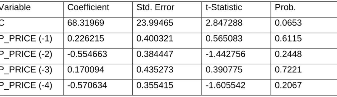
Table 17. four period lagged potato price(Q1-Q4) ... 36
Table 18. Measuring forecast accuracy ... 39
ix LIST OF FIGURES
Figure 1. Potato production in 16 regions, Source: Potato South Africa ... 12
Figure 2. percentage of producers versus size of planting hectares-2016 crop year .... 12
Figure 3. Fluctuating Residual for potato price form year 2006 to 2016 ... 23
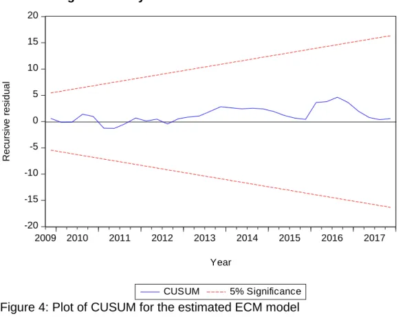
Figure 4. Plot of CUSUM for the estimated ECM model ... 36
Figure 5. Forecasted quarterly potato price from 2018q1 to 2019q4(10kg) ... 37
Figure 6. Forecasted quarterly potato price from 2006q1 to 2019q4(10kg) ... 38
x LIST OF ACRONYMS
DAFF Department of Agriculture, Forestry and Fisheries FAO Food and Agriculture Organization
WTO World Trade Organization IMF International Monitory Funds
IFPRI International Food Policy Research Institute
OECD Organization of Economic Cooperation and Development UNCTAD United Nations Conference on Trade and Development WFP World Food Programme
UN HLTF United Nations High-Level Task Force IFAD International Food Policy Research BC Before Christ
PSA Potato South Africa
CIP International Potato Center
NDA National Department of Agriculture SAWE South African Weather Service
NAMC National Agricultural Marketing Council
ARCH Autoregressive Conditional Heteroscedasticity
GARCH Generalized Autoregressive Conditional Heteroscedasticity CV Coefficient of Variation
AR Autoregressive DF Dickey-Fuller
ADF Augmented Dickey-Fuller ECM Error Correction Model
VECM Vector Error Correction Model VAR Vector Autoregression
xi ADL Autoregressive Distributed Lag
RMSE Root Mean Square Error MPE Mean Pricing Error
MAPE Mean Absolute Pricing Error
MARPE Mean Absolute Relative Pricing Error Kg Kilogram
R Rand Ha Hectare R Rand
BFAP Private Farmers Assistance Program Q1 First quarter
Q2 Second quarter Q3 Third quarter Q4 Fourth quarter
NPK Nitrogen, Phosphorus and Potassium Rwf Rwandan Francs
Usd United States Dollar SQRT Square Root
CUSUM Cumulative Sum
AIC Akaike Information Criterion SC Schwarz Criterion
HQ Hannan-Quinn Information Criterion LR Likelihood Ratio
FPE Final Prediction Error
1 CHAPTER ONE
INTRODUCTION 1.1 Background
An unacceptably high number of people suffer from food and nutrition insecurity in the world. Multiple episodes of food crises in the last decade have made the situation worse (Kalkuhl et al., 2017). During periods of excessive price volatility, it is the poor and vulnerable population that are mostly affected. In South Africa, majority of the people particularly those residing in rural areas depend on agriculture for their living. Potato industry has become an important food provider and this has then led to the establishment of Potatoes South Africa that operates as an industry. The industry aims to support potato producers within the regional context in South Africa to ensure viability of potato industry.
However, price fluctuations have become large and unexpectedly volatile and this can have a negative impact on the food security of consumers, farmers and the entire country.
Since 2007, the agricultural commodity markets have experienced extreme price fluctuations more and more frequently (Kalkuhl et al., 2017). Food prices today remain high, and are expected to remain volatile (FAO, 2009). The price volatility of agricultural commodities has been exceptionally high during the commodity boom of 2006-2008 (Schnepf, 2008). Food prices increased between late-2006 and mid-2008 to their highest level in thirty years, fell sharply through 2009 then regained their 2008 peak in late 2010- early 2011 FAO (2012). Since the high record of food prices in 2009, potato prices have traded softer over the year 2010-2012 in a relatively constant band of R23 to R26 per 10 kg bag BFAP (2012). Due to a shorter cropping season in 2013, prices traded higher than in 2012 by an annual average market price of R31 per 10 kg BFAP (2013). For 2014, prices traded around R36 per 10kg bag BFAP (2014). The price decreased in 2015 from R36 to R33 and Potatoes South Africa (PSA) reports that potatoes reached a record price of R60 per 10kg on 19 January 2016, the highest average weekly price on record for potatoes (DAFF, 2016).
2 Potato is the world’s number one non-grain food commodity FAO (2010) and the fourth largest crop in terms of fresh produce after rice, wheat and maize (Sopib, 2011). Potatoes have also established itself over time as a worthy alternative in the staple food category PSA (2015) and an excellent crop in the fight against hunger and poverty. The potato was first domesticated in the region of modern-day southern Peru and extreme north-western Spooner et al. (2005) between 8000 and 5000 B.C. it has since spread around the world and become a staple crop in many countries. It is generally believed that potatoes entered Africa with colonists, who consumed them as a vegetable rather than as a staple starch (Ornelas, 2000).
According to legend, the first potatoes for planting purposes in South Africa came from Holland to provide food for mariners visiting the Cape. Since then the potato industry has grown to become one of the important food providers in South Africa (NDA, 2003).
Potatoes play a role in the South African economy in terms of its contribution to the gross domestic product (PSA, 2015). Taking the combined value of the field crop and horticultural sectors, potatoes is the fifth biggest agricultural sub-sector, and this when merely between 50 000 and 54 000 hectares are used for potato production (PSA, 2015).
Potatoes yield food that is more nutritious more quickly, on less land and in harsher climates than most other major crop (Wikinson, 2001). Potato crops are also highly adaptable to a wide variety of farming systems. Their short and highly flexible vegetative cycle, which brings yields within 100 days, fits well with double cropping and intercropping system FAO (2010). South Africa Potatoes are grown all year-round owing to the country’s unique geography and climate. Potatoes are produced all over South Africa in different climatic regions. This results in a continuous supply of potatoes throughout the year (DAFF, 2013).
In South Africa, potatoes are not categorised as a seasonal product. Due to the different climatic conditions, e.g. temperature, rainfall and soil type. In the 16 production regions, potatoes are planted and marketed at different times by the relevant regions to ensure a continuous supply of fresh potatoes throughout the year. Potatoes are grown mainly
3 under irrigation, but in some of the production regions potatoes are grown successfully under dry land conditions. As potato is a cool climatic crop, most production regions takes place in a climate not optimal for potato production. Temperatures in excess of 300C and fluctuating daily temperatures cause stress in plants, which in turn limits yield potential of even the best adapted cultivars (PSA, 2015).
1.2 Problem statement
Gilbert and Morgan (2011) defined price volatility as the quantitative measure of the directionless extent of the variability of the price of a given asset. FAO (2011) purely gave a descriptive sense of volatility as a variation in economic variables over time.
The main problem this study attempts to analyse is the extreme potato price volatility that is more likely to hurt the consumer’ pockets. Poor households spend a large amount of their total income, often more than 60% on food, so a given variability in food prices has a large effect on purchasing power (FAO et al., 2011a and FAO et al., 2011b). Food price increases naturally become an issue to poor consumer resulting in them cutting expenditures on other domains such as health or on the quality of food, which ultimately can contribute to micronutrient deficiencies (Kalkuhl et al., 2017). Many consumers are being forced to take only the essentials from the store shelves. Shoppers have noticed a sharp increase in the price of basic food staples. The cost of potatoes has pushed the vegetable out of reach for the poorest of the poor (Epstein, 2016).
The 2015 harvest delivered 250 million bags of potato as reported at the end of November 2015. An oversupply of an additional 12, 9 million bags of potatoes was made (Elsenburg, 2016). However due to the 2016 heat waves resulting in dry hot weather the quality of potatoes was affected. This created a limited supply of good quality potatoes and resulted in a price increase above normal seasonality (Willemse et al., 2015). According to Hartigh (2016), prices have more than doubled in 2016 from a year earlier and the price for 10kg potatoes packet has increased from R33.30 by January 2015 to R73.32 by January 2016.
4 The extreme price volatility means insecurity and financial risks for all the commercial operators involved (Wellard, 2012). In 2016, seed potato producers would not sell their seed potatoes because the commercial producers were discouraged to plant potatoes due to lack of soil moisture. This result in high production costs, which affect potato production, pushing up potato price that have already increased. Yet again, the poor were mostly affected (Willemse et al., 2015). This study, therefore, attempts to examine the various factors that are responsible for potato price volatility in South Africa.
1.3. Motivation
The rationale behind the study is due to the enormous potato price hike experienced in year 2016, which was widely felt by Farmers, consumers and entire country. The study analyses the possible cause of the recent potato price spike. The study also provides a forecast for potato price for the period 2018-2019 to determine the level of potato price volatility. The results from the study will also assist policy makers to come up with strategies to curb potato price volatility.
1.4 Aim of the study
i. The aim of the study is to analyse potato price volatility in South Africa.
1.5 Study objectives
The specific objectives of the study were to:
i. Determine the variability of potato price from 2006 to 2017.
ii. Identify and analyse the determinants of potato price change in the market.
iii. Forecast potato price from 2018 to 2019.
1.6 Hypotheses
i. Potato price volatility cannot be influenced by volatility of independent variables.
ii. Potato price cannot be cointegrated with the independent variable
5 CHAPTER TWO
LITERATURE REVIEW 2.1 Introduction
This chapter presents a review of some of the studies that have been undertaken in the past. The chapter begin by giving a definition of price volatility and then outline what volatility is. The study assessed the recent causes of potato price volatility in South Africa, and then continued to assess the determinants or factors affecting potato price volatility.
2.2 Defining price volatility and volatility
Price Volatility simply means the degree of change in the price of a stock over time.
Some investment opportunities have a high degree of change, or high price volatility, and some have a low degree of change, or low-price volatility. The concept of price volatility on agriculture describes how frequently the prices of agricultural products change over time, both upwards and downwards. While some variation in prices is considered to be a normal aspect of well-functioning markets, volatility becomes problematic when price movements are large and unpredictable.
High levels of price volatility can create financial risks for farmers, since their incomes will be less predictable and can be threatened by sudden price drops. Price volatility also reduces capacities for long-term investments, particularly for young farmers. Moreover, increases in agricultural prices can reduce the ability of lower-income households to fulfil their basic needs, especially in developing countries, as the cost of food represents a large share of their income (Tropea and Devuyst, 2016).
Volatility is the conditional standard deviation of the underlying assets return (Grek, 2014). Volatility is usually referred to as a measure of variability. In financial time series, when we say that the market is volatile, we mean that there is uncertainty on investments.
High volatility means uncertainty in the periods of time while in financial time series, high volatility means that the investments carry high risk of losses (Serrano et al., 2011).
6 2.3 Factors affecting potato price volatility
The prices of potatoes are highly fluctuating. There are number of factors that explain why agriculture is confronted with higher levels of price volatility than other economic sectors. The factors which affect the prices of potatoes are mainly fluctuations in area of production, weather, production level and yield, irrigation facility, demand for potato in cities and from food processing industries, input cost for potato cultivation, transportation charges, labour availability during planting and harvesting, storage capacity and stock position in cold storage (Mumtaz et al., 2015). The following are some of the factors affecting potato price volatility.
2.3.1 Weather condition.
Climate change (extreme weather conditions) is one of the root causes for the recent high and volatile food prices (Waschkeit et al., 2011). Climatic factors have indisputably contributed to the price rises in 2007/2008 (FAO et al., 2011). Weather shocks are considered to be one of the important sources of variability in agricultural commodity prices (Morgan and Gilbert, 2010). Disasters such as drought and flooding can cause catastrophic damage to crop (Mirzabaer and Tsegai, 2012). Drought is the most common cause of stress in potato (Onder et al., 2005). Drought stress is important and farmers in the east of Ireland have to flood irrigate potato fields to ensure adequate yields.
Given that, an increased seasonality of water supply is predicted (Sweeney and Fealy, 2001). Vulnerability of potato to drought has been attributed mainly to the crop’s shallow root system and low capacity of recuperation after a period of water stress (Iwama and Yamaguchi, 2006).
Climate change will provoke some adjustment of production patterns around the world, as well as increased risks of local or regional supply problems that could add to future volatility (FAO et al., 2011).
Potatoes are essentially a crop that thrive in cooler conditions, despite being very susceptible to frost (Bill, 2012). According to PSA (2014), the potato is a temperate crop
7 and is sensitive to water and high temperature stresses. Higher daily temperatures and changes in rainfall increases crop stress, and may render production areas less suitable for potato production, resulting in lower tuber yields and quality. Hijmans (2003) studied the effect of climate change on global potato production between year 1961-1990 and 2040-2069.The study showed that temperature increase is smaller when changes are weighted by the potato area and particularly when adaptation of planting time and cultivars is considered a predicted temperature increase between 1 and 1.4 C. For this period, global potential potato yield decreased by 18% to 32% without adaptation and by 9% to 18% with adaptation.
Extreme weather events, such as high intensity rainfall events, can be damaging to potatoes. Waterlogged conditions in the soil, particularly in summer rainfall areas, can result in tubers rotting, as these are optimal conditions for development of soft rot and blackleg (Steyn et al., 2014).
2.3.2 Market factors
In the short-term, because the market fundamentals of supply and demand are inflexible towards agricultural products, reconciling these two forces can be hard when it comes to such products. Demand is rather fixed because food is a basic human necessity, while supply is unable to adapt quickly because food takes time to be produced. As a result, even small changes in agricultural supply or demand can cause large variations in prices, causing permanent market instability. Apart from these microeconomic fundamentals, changes in macro-economic factors, such as exchange rates and oil prices, can also have a substantial influence on food prices.
In their study, Mwangi et al. (2013) on “Effect of market reforms on Irish potato price volatility in Nyandarua district” an autoregressive econometric technique was used to examine the effects of the implementation of market reform policies by the Kenyan government on the Irish potato sub-sector. The results indicated that the implementation of market reform policies favoured the Irish potato producers but made the consumers worse off. The study showed that price volatility in the Irish
8 potato sector is as a result of factors having effects on supply and demand. The supply increased as a result of increased production while the demand rose due to increase in population, rapid urbanization and change in tastes and preferences.
However, the variability in value of production was found to be a major contributor to Irish potato price volatility because production follows the natural rainfall pattern.
Guenthner et al. (1991) conducted study to determine factors affecting the demand for potato product in the United States. The study stated that the economic theory suggests the demand for potato is influenced by price of complimentary product, consumer debt, change in consumer tastes and preferences, own price and population. The study showed that explanatory variables had opposite impact on the demand for different potato products. The amount of income that consumers have available to spend was found to be the most important variable among all other variables.
Thorne (2012) studied potato price as affected by supply and demand factors: An Irish case study, the main objective of the paper was to evaluate the factors influencing potato price formation at farm level in Ireland over the period 1992 to 2011. The study used OLS regression to determine relationship between yearly potato price, production of potatoes produced and consumption of potatoes produced nationally.
The results indicated that potato prices decrease with increasing volumes and increase with increasing consumption levels. The estimated demand function for potatoes in Ireland has shown a structural break during the last two decades. While the demand for potatoes decreased, the price adjustments to changes in demand decreased significantly. Hence, it can be concluded that the demand for potatoes has become notably more price elastic.
Goodwin et al. (1988) analysed factors affecting fresh potato price in selected terminal markets. The general objective of this study is to identify and assess factors affecting fresh potato price at terminal markets. The model specification was builds on the theoretical framework of Ladd and Suvannunt and the hedonic price.
9 2.3.3 Production cost
Mumtaz et al. (2015) studied the determinants of potato prices and its forecasting: A case study of Punjab, Pakistan. The objective of this study was to analyse various factors that affect the prices of potatoes in Punjab over a period of time. The study used general empirical model for the price of fresh potato that consist of production area, production costs, price of crude oil, support price and temperature as independent variables and the study concluded that the cost of production has the major impact on the prices of potatoes in Punjab. For forecasting SARMA model has been applied since the prices of potato have a seasonal trend.
Nsabimana et al. (2015) used GARCH and VECM in forecasting price of Irish potatoes volatility from 2007 – 2015. The result showed that price of Irish potatoes is highly peaked and moderately skewed. The volatility of fertilizers especially NPK1515 does not granger cause the volatility of Price of Irish potatoes. The volatility of pests does not have a long run associationship with the volatility of Irish potatoes and the exchange rate doesn’t granger cause the volatility of Irish potatoes in the studied areas.
In their study, Duyan and Tagarino (2015) on “Price volatility of selected high value vegetables in Cordillera administrative region, Philippines” focused on the price trend of cabbage, carrot and potato for the period of 2002 to 2011. They found that the prices of the selected vegetables involving farm, local retail and Metro Manila retail were erratic for the whole periods covered and that there was no consistent surge and decline of prices observed except for potato that exhibits increasing trend from 2005 to 2011. Vegetable prices specifically farm and retail are affected significantly by several factors such as the weather conditions including rainfall amount and temperature, the production area, and volume of imports. The relationship of the selected variables to the vegetable prices indicates positive slight to very high correlation.
Habyarimana et al. (2014) conducted the study on Food price volatility in Rwanda to explore the long and short run relationship between food prices volatility and forecast
10 food prices volatility in Rwanda using Vector Autoregressive (VAR) Model for Multivariate Time Series. The paper used six agriculture commodities (Sorghum, Maize, Rice, Wheat, Beans, and Irish Potato), to conclude on which variables can help to explain food price volatility in the last seven years. The paper showed that forecasted food price in one commodity can be gradually attributed to the past price volatility of the same commodity and that of others. The granger causality test showed that there exists food prices granger causality in the selected food commodities. Thus, the impulse response analysis showed that shock to the price of one food commodity create smaller, but significant response and temporary oscillations in other food commodities and itself but which impact on other food process do not persistent and that their effects eventually die out.
11 CHAPTER THREE
RESEARCH METHODOLOGY 3.1 Introduction
This chapter describes methodology on data collection. A secondary data was collected from Potatoes South Africa (PSA) and South African Weather Service (SAWS). Eviews statistical tool was used to run and analyse the data. Data collected was for quarterly potato price (PP), quarterly number of hectares planted (HA), quarterly rainfall (R) and quarterly temperature (T) level from year 2006 to 2017 making the total observation of 48.
It further gives an overview background description on the study area which covers all provinces of South African potato producing regions. The first part of methodology in this chapter measures the variability of potato price,followed by introducing the element of modeling potato price volatility. The second part introduces the VECM model used to examine relationship between potato price as the dependent variable in this study and the various independent variables. Later in this chapter, the study provides forecasting of potato price using ECM model.
3.2 Potato production regions
Potatoes are produced from sixteen production regions which are spread throughout South Africa. The main producing regions are situated in the Limpopo, Free State, Western Cape, Mpumalanga, Kwa-zulu Natal and Eastern Cape DAFF (2012). South African potato production is mainly under irrigation. Potatoes are produced without supplementary irrigation (dryland) only during spring and early summer plantings in regions with a cool temperate climate and a proven reliable summer rainfall such as in the Mpumalanga Highveld and Eastern Free State DAFF (2012).
12 Figure 1: Potato production in 16 regions
Source: Potato South Africa
Figure 1, shows the potato production in 16 regions, where potatoes are produced both under irrigation and under dry land.
Planting of potatoes is done almost throughout the year in different regions of South Africa consequently resulting in continuous access to fresh potatoes. The season is divided into two production periods. The early crop is planted from January to March and the main crop is planted from April to August. The months of November and December are avoided because of high temperatures combined with long day lengths, which are not conducive for planting.
13 Figure 2: The percentage of producers versus size of planting in hectares in 2016
Source: Potato South Africa
Figure 2 indicate the percentage of producers versus size of planting in hectares in 2016 crop year across all planting regions in South Africa. The high percenatge of producers contributing about 53% planted potatoes on less than 51 ha and 10% producers planted their potatoes on more than 200 ha.
3.3 Data collected and source of data Table 1: Data collection and source
Data collected (all in Quarterly) Source of the data
Potato price from 2006q1-2017q4 (PSA) Potato South Africa Number of hectares planted from 2006q1-
2017q2
(PSA) Potato South Africa
Rainfall from 2006q1-2017q2 (SAWE) South African weather service Temperature from 2006q1-2017q2 (SAWE) South African weather service
14 3.4 Methods of data analysis
The study used coefficient of variation to measure variability of potato price from 2006 to 2017. To analyse potato price volatility from year 2006 to 2017 the study used the Autoregressive Conditional Heteroscedasticity model (ARCH) and the General Autoregressive Conditional Heteroscedasticity model (GARCH). The study, firstly described clustering volatility followed by ARCH and GARCH effect in the series. The graph was used to describe fluctuating residuals of potato price from 2006 to 2017. Also the tables were used to describe ARCH and GARCH effect. The GARCH effect used mean equation model to test as to whether volatility of independent variables have an influence on potato price volatility. ARCH effect used variance equation model to analyse volatility of independent variables on potato price volatility. Diagnostic check was performed to check whether the estimated model has ARCH effect and serial correlation or not.
Augmented Dickey Fuller test was used to check whether the time series is stationary or non-stationary. When time series are integrated of the same order I(1),the study run Johansen test of cointegration using both trace and eigenvalue test to check if variables have a long run relationship. Having found variables that are cointegrated, the study proceeds to use vector error correction model (VECM) to determine short run relationship between potato price and various variables. However, before performing cointegration test and VECM modeling, the study undertaken VAR lag order criteria to determine optimal number of lags to use in the system equation. Granger causality was used to examine the causal relationship amongst the variables. The residual diagnostic was used test to check if there is serial correlation. The cumulative sum (CUSUM) test was used to assess the stability in the coefficient of estimated ECM.ECM model was also used for forecasting.
3.4.1 Measures to evaluate volatility
The coefficient of variation was used to evaluate the quarterly potato price volatility. The coefficient of variation (CV) is defined by (Brian, 1998) as the ratio of standard deviation 𝛿 to the mean 𝜇 and it is a useful statistical tool for comparing a degree of variation from
15 one data series to the other. The coefficient of variation is a simple unconditional measure of price variability. The following coefficient of variation formula was used.
V = 𝜎
𝜇 =
√1
𝑛∑𝑛𝑖=1(𝑥1 − 𝜇)
𝜇 (1)
Where: v been the coefficient of variation, 𝜎 been the Standard deviation for potato price,𝜇 are the Mean prices for potato and 𝑥1 been observed potato prices.
3.4.2 Modeling Volatility
This study attempted to model the volatility of quarterly potato price and the independent variables using both ARCH/GARCH model proposed by Engle (1982) and Bollerslev (1986) models respectively;
3.4.2.1 Clustering volatility
In order to run ARCH model, the study, firstly describe clustering volatility and ARCH effect in the series. Clustering volatility was analysed by checking if there is an evidence of high or low volatility in the time series. When there is evidence of clustering volatility and ARCH effect in the time series, the study proceeds to perform ARCH and GARCH model.
3.4.2.2 The (ARCH) Autoregressive Conditional Heteroscedasticity Model
The autoregressive conditional Heteroscedasticity is a statistical model for the time series data that describes the variance of the current error term as a function of the actual sizes of the previous time period’ error terms Engle (1982). The ARCH specification helps to focus on the mean and the variance of time series, which are useful to understand the magnitude of volatility in time series data. Engle (1982) offered modeling conditional volatility by using ARCH process; which is in simple words a function of lagged squared residuals, and the general form of the model is:
16 𝑦2𝑡= 𝛼0 + 𝛼1𝜀2𝑡−1+…+ 𝛼𝑞𝜀2𝑡−𝑞
That is:
𝑦2𝑡 = 𝛼0 + ∑𝑞𝑗=1𝛼1𝜀2𝑡−𝑖 (2)
Where𝛼0 is a mean,𝛼1is conditional volatility and 𝜀𝑡−1 is white noise representing residuals of time series and 𝑦2𝑡 is conditional variance.
3.4.2.3 The (GARCH) General Autoregressive Conditional Heteroscedasticity Model
In the ARCH model, there are certain limitations that may result in an insufficient estimation on volatility however, Bollerslev (1986) proposed a modified form through Generalized ARCH (GARCH) that will permit a longer memory and a more flexible lag structure to overcome those limitations. GARCH is a statistical model used in analysing financial time series data. The model was estimated in the following form:
𝑦2𝑡= 𝛼0 + 𝛼1𝜀2𝑡−1 +…+ 𝛼𝑞𝜀2𝑡−𝑞 + 𝛽1𝑦2𝑡−1 +…+ 𝛽𝑝𝑦2𝑡−𝑝 That is:
𝑦2𝑡= 𝛼0 +∑𝑞𝑗=1𝛼1𝜀2𝑡−𝑖 + ∑𝑝𝑖=1𝛽𝑖 𝑦𝑡−𝑖(3)
Where 𝑦2𝑡 is conditional variance, 𝛼0 is a mean, ∑𝑞𝑗=1𝛼1𝜀2𝑡−𝑖 is the ARCH effect and
∑𝑝𝑖=1𝛽𝑖 𝑦𝑡−𝑖 is GARCH effect.
The GARCH (p,q) model with constraint,𝛼0 ˃ 0,𝛼1≥ 0, i= 1,…q and 𝛽𝑖 ≥ 0, 𝑗 = 1…,p with,𝛼1 + 𝛽𝑖 ˂ 1, 𝛼1and 𝛽𝑖 are ARCH and GARCH parameters respectively, unconditional variance𝑦2𝑡 evolve over time t.
17 3.4.2.4 Diagnostic check
The study performed heteroscedasticity and serial correlation tests to check whether the estimated model has ARCH effect and serial correlation or not. If there exist the evidence of heteroscedasticity and serial correlation, the results drawn from model will not be reliable. Model may be poorly defined.
3.4.3Unit roots tests
Unit root test tests whether a time series variable is non-stationary and possesses a unit root. The test was carried out to feature some stochastic (such as random walks) that can cause problems in statistical inference involving in the series model. The study used Augmented Dickey-Duller (1979) method to test for the existence or non-existence of unit roots in the variables used in estimating the South African potato price volatility namely;
potato price, number of hectares planted, rainfall and temperature level. If the variable is non-stationary, it need to be differenced until it become stationary. If it is differenced once, it is said to be integrated of order one I(1).
∆𝑃𝑃𝑡 =𝛼0 + 𝛾𝑃𝑃𝑡−1 + 𝛼2𝑡 + ∑𝑝𝑖=1𝛿𝑖 ∆𝑃𝑃𝑡−𝑖 + 𝑢𝑡
∆𝐻𝐴𝑡 =𝛼0 + 𝛾𝐻𝐴𝑡−1 + 𝛼2𝑡 + ∑𝑝𝑖=1𝛿𝑖 ∆𝐻𝐴𝑡−𝑖 + 𝑢𝑡
∆𝑅𝑡 =𝛼0 + 𝛾𝑅𝑡−1 + 𝛼2𝑡 + ∑𝑝𝑖=1𝛿𝑖 ∆𝑅𝑡−𝑖 + 𝑢𝑡
∆𝑇𝑡 =𝛼0 + 𝛾𝑇𝑡−1 + 𝛼2𝑡 + ∑𝑝𝑖=1𝛿𝑖 ∆𝑇𝑡−𝑖 + 𝑢𝑡
Where: 𝛼0 is a vector of deterministic term (constant, trend etc.), 𝛼2 is the coefficient on a time trend series, 𝛾 is the coefficient of 𝑦𝑡−1, ∆𝑦𝑡−𝑖 are the changes in lagged values, 𝑦𝑡−1 are lagged values of order one of 𝑦𝑡, P is the lag order of autoregressive process, 𝑢𝑡 is an error term.
Under null hypothesis 𝑦𝑡 is I (1) which implies that 𝛿 = 0
18 3.4.3.1 Testing for cointegration
Das (1973) Cointegration is a statistical property possessed by some time series data that is defined by the concepts of stationarity and the order of integration of the series.
If there exists a stationary linear combination of non-stationary random variables, then the variables combined are said to be cointegrated and may have a stable long run relationship. The study used Johansen procedure to test for cointegration relationship amongst variables. The VAR Lag order selection process was undertaken in order to determine the optimal number of lags to use in the cointegration and VECM equation.
Johansen’s procedure
The study firstly establishes the order of integration of the modelled variables to determine whether two variables are cointegrated. This was done by performing unit root test as indicated in section 3.4.3. If the two variables are integrated of the same order, then the study proceed to estimating the long run equilibrium relationship using Johansen test of cointegration. The Johansen test can be seen as a multivariate generalization of the augmented Dickey Fuller test Dwyer (2015). This test permits more than one cointegrating relationship so is more generally applicable than the Engle–Granger test which is based on the Dickey–Fuller (or the augmented) test for unit roots in the residuals from a single cointegrating relationship Davidson (2000).The Johansen test is a VAR- based cointegration test. The general form of the VAR (p) model, without drift, was given by:
𝑦𝑡= µ+𝐴1𝑦𝑡−1+. . . + 𝐴𝑘 𝑦𝑡−𝑘 + 𝜀𝑡
This VAR can be re-written as
∆𝑦𝑡 = µ + П𝑦𝑡−1 + ∑𝑘−1𝑖=1 П𝑖∆𝑦𝑡−𝑖 + 𝜀𝑡(4)
Two types of Johansen test, the trace and the eigenvalue were used to determine if there exist long run relationship amongst variables.
19 Trace test
The trace test examines the null hypothesis of k cointegrating vectors against the alternative hypothesis of n cointegrating vectors. The test statistic was given by
𝐽𝑡𝑟𝑎𝑐𝑒 = -T ∑𝑛𝑖=𝑘 +1𝖨𝚗(1 − 𝜆̂𝑖) (5)
Maximum Eigenvalue Test
The maximum eigenvalue test examines the null hypothesis of k cointegrating vectors versus the alternative 𝑘 + 1 vectors. Its test statistic was given by,
𝐽𝑚𝑎𝑥 = - T 𝖨𝚗(1 − 𝜆̂𝑘+1) (6)
Where T is number of observation,𝜆̂𝑖 is the 𝑖𝑡ℎlargest canonical correlation
If the variables are cointegrated, the study proceed to run Vector Error Correction Model to determine long run and short run relationship.
3.4.3.2 Vector error correction model (VECM)
The cointegrating regression so far considers only the long-run property of the model, and does not deal with the short-run dynamics explicitly. The study used vector error correction model (VECM) to describe short-run dynamics of the cointegrating variables respectively. VECM can be used to granger causality when the variables are cointegrated and have unit roots. Granger causality is a statistical concept of causality that is based on prediction (Seth, 2007). The study used Wald tests to check if current value of potato price (PP) was caused by past value of number of hectares planted (HA) and rainfall level (R) respectively:
∆𝑃𝑃𝑡 = α + 𝛿𝑡 + 𝜆𝑒𝑡−1 + 𝛾∆𝐻𝐴𝑡−1 + . . . +𝛾∆𝐻𝐴𝑡−𝑝
+ 𝜔1∆𝐻𝐴𝑡−1 + . . . + 𝜔𝑞∆𝐻𝐴𝑡−𝑞 + 𝜀𝑡 (7)
∆𝑃𝑃𝑡 = α + 𝛿𝑡 + 𝜆𝑒𝑡−1 + 𝛾∆𝑅𝑡−1 + . . . +𝛾∆𝑅𝑡−𝑝
20 + 𝜔1∆𝑅𝑡−1 + . . . + 𝜔𝑞∆𝑅𝑡−𝑞 + 𝜀𝑡 (8)
HA Granger causes PP if past values of HA have explanatory power for current values of PP.
3.4.3.3 Diagnostic check
The study adopted residual diagnostic test to check if there is serial correlation in the model or not, the results are displayed on a table form. It further used cumulative sum (CUSUM) test to check whether the model is stable or not.
3.4.4 Forecasting with ECM model
The study used out of sample forecasts. ECM model was used for forecasting since its based techniques result in lowest forecast error in long run forecasting.
To forecast ∆𝑋𝑡+ 𝜏 . The forecast of 𝑋𝑡+ 𝜏(𝜏 is the step ahead) are obtained recursively:
𝘟̂𝑡+ 𝜏 = ∆𝘟̂𝑡+ 𝜏 + 𝘟̂𝑡+ 𝜏−1 (9) 3.4.4.1 Forecasting accuracy+
After forecasting, the standard statistical measures such as Mean pricing error (MPE), mean absolute pricing error (MAPE), mean absolute relative pricing error (MARPE), and root mean squared error (RMSE) were calculated to determine the effectiveness of the forecasts.
This study focused primarily on RMSE, which gives a measure of the magnitude of the average forecast error, as an effectiveness measure. The RMSE depends on the scale of the dependent variable. The RMSE may be estimated as:
RMSE = √1
𝑛∑𝑛𝑖=1(𝑆1 − 𝐹𝑃𝑖)2(10)
21 And Theil’s inequality coefficient (U)
U =
√1
𝑛∑𝑛𝑖=1(𝑆1 − 𝐹𝑃𝑖)2
√1
𝑛∑𝑛 𝑆21
𝑖=1 + √𝑛1∑𝑛 𝐹𝑃21 𝑖=1
(11)
Where 𝑆1 , is the actual potato price.
𝐹𝑃𝑖 , is the future potato price.
3.5 Table 2: Analysis of objectives
Study objectives Model Reasons for model
To determine the variability of potato price from 2006 to 2017
The (ARCH)
Autoregressive Conditional Heteroscedasticity and (GARCH) General
Autoregressive Conditional Heteroscedasticity model
To model conditional volatility
To identify and analyse the determinants of potato price change in the market
(VECM) Error Correction Model
Addresses both short run dynamics and long run equilibrium relationship amongst variables.
To forecast potato price from 2018 to 2019
(ECM) Model Forecast results in lowest forecast error in long run forecasting.
22 CHAPTER FOUR
RESULTS AND DISCUSSION
4.1 Introduction
This chapter presents the results of the analyses of potato price volatility in South Africa.
The chapter begins by measuring variability of potato price from year 2006 to 2017. ARCH and GARCH model were run to determine volatility in the series. Diagnostic check was performed to check the Heteroscedasticity and serial correlation. Pretesting for unit roots test was carried out using Augmented Dickey fully test to determine the number of integration order amongst economic variables. Johansen procedure tested long run relationship amongst variables. The VECM results for both long run and short run relationship between potato price and various independent variables were analysed and discussed. The study further forecasted potato price using ECM.
4.2 Measures to evaluate volatility Table 3: Coefficient of variation
Year Standard deviation(𝜎) Mean( 𝜇) Coefficient of variation (CV)
2006 2,265809 17 0,132639*100= 13.26%
2007 7,338585 22 0, 33361*100= 33.36%
2008 3,605065 21 0,173759*100= 17.38%
2009 4,903363 31 0,155687*100= 15.57%
2010 4,371372 26 0,166038*100= 16.60%
2011 4,837509 26 0,186076*100= 18.61%
2012 4,597633 26 0,174103*100= 17.41%
2013 7,748931 35 0, 21933*100= 21.93%.
2014 2,996636 34 0, 08708*100= 8.70%
2015 3,717028 28 0,131973*100= 13.19%
2016 7,277465 48 0,152687*100= 15.26%
2017 4,981003 26 0,191577 * 100=19.15%
23 Table 3 indicate potato price variation for each year from 2006 to 2017. A data set of 2007 has more variability, giving the coefficient of variation of 31.361% as compared to 13.2636% of 2006. Although 2008 has low coefficient of variation of 17.3579% compared to 31.361% of 2007, however when comparing 2008 with 2009 which is given by 15.5687%, 2008 has high variation of coefficient. The study evident that when dispersion is lower in the first data set, the second dataset will be higher and vice versa. The lower coefficient of variation indicates a decrease in volatility whereas the higher coefficient of variation indicates an increase in volatility. In their study,Vigila et al. (2017) observed a large variation in the prices of potato in four major states namely, Maharashtra, Tamil Nadu, Uttar Pradesh and Gujarat between years 2005-2016. The results showed that among the four states, Tamil Nadu (TN) had a smaller variation in the potato price of 35.49% of CV than other three states.
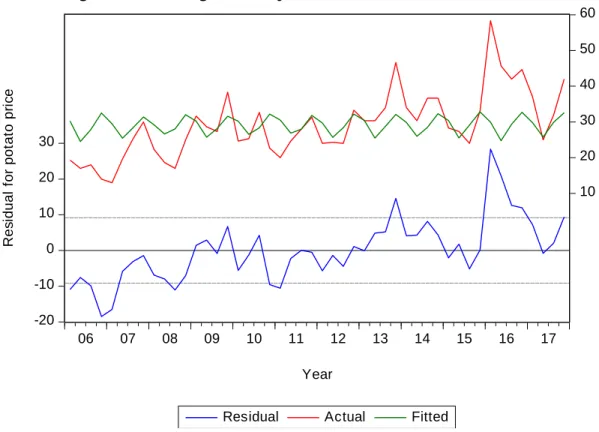
4.3Testing for clustering volatility
-20 -10 0 10 20 30
10 20 30 40 50 60
06 07 08 09 10 11 12 13 14 15 16 17
Residual Actual Fitted Year
Residual for potato price
Figure 3: Fluctuating Residual for potato price form year 2006q1 to 2017q4
24 Clustering volatility means that the period of low volatility followed by period of high volatility for a long period of time and vice versa. From figure 3, the results show that from 2006(q1) to 2006(q4) low volatility was followed by another low volatility for a long period and volatility started to peak from 2007(q1) to 2007(q4), meaning period of high volatility was followed by period of high volatility. The study noticed period of low volatility from 2008(q1) to 2008(q2), period of high volatility peaks again from 2008(q3) to 2009(q3). In 2009(q4) to 2012(q3) there was an evidence of low volatility. This was supported by Nsabimana et al. (2015) in their study on forecasting price of Irish potatoes volatility using GARCH and VECM Models in Rwanda were it was observed that the Irish potatoes goes by decreasing from +32% in 2010; + 21.1% in 2011 and +13.4% in 2012 up to -4.2% in 2013. It shot up again to high volatility in 2014(q4) to 2014(q3). 2014(q4) to 2015(q4) the period of low volatility was observed on figure 3 and period of high volatility was followed from 2016(q1) to 2016(q4). In 2017(q1) to 2017(q4), there was an evidence of low volatility. The study concludes that there is clustering volatility, therefore the study proceeds to run ARCH model. Nsabimana et al. (2015) concluded that there was an indication of clustering volatility price of Irish Potatoes because on figure 2, the graph showed that the high volatility tends to be followed by high volatilities and low volatility was followed by low volatility. The study proceeds to run ARCH model
4.3.1 Testing for ARCH effect Stating null hypothesis as:
𝐻0: There is no ARCH effect 𝐻1: There is ARCH effect
Table 4: Heteroscedasticity Test: ARCH
F-statistic 9.540098 Prob. F (1,41) 0.0036
Obs*R-squared 8.116807 Prob. Chi-Square (1) 0.0044
Under null hypothesis stating that there is no ARCH affect, the study observed results from table 4 indicating that prob.chi-square is 0.0044 meaning is less than 5%, therefore;
we can reject null hypothesis, there is ARCH effect. Therefore, the study have valid
25 reason to run ARCH model because there is clustering volatility observed from figure3 and ARCH effect was tested on table 4.
4.2.4 Testing GARCH effect Stating null hypothesis as:
𝐻0: There is no GARCH effect 𝐻1: There is GARCH effect
Table 5: Mean equation and variance equation model: GARCH affect GARCH = C(7) + C(8)*RESID(-1)^2 + C(9)*GARCH(-1)
Variable Coefficient Std. Error z-Statistic Prob.
@SQRT(GARCH) 1.415233 0.741541 1.908502 0.0563
C 65.41427 6.585095 9.933687 0.0000
R_RAINFALL_MM 0.003024 0.033417 0.090491 0.0092 HA_HECTARE -0.000160 4.79E-05 -3.343709 0.0008 T_TEMP -0.198444 0.180027 -1.102303 0.2703
C 10.59822 8.238053 1.286496 0.1983
RESID (-1) ^2 -0.907232 0.703838 1.288979 0.1974 GARCH (-1) 1.078374 0.021077 51.16459 0.0000 T-DIST. DOF 2.032925 0.024201 84.00289 0.0000
R-squared 0.841806 Mean dependent var 28.69318
Adjusted R-
Squared 0.820991 Mean dependent var 9.287120
S.E. of regression 3.929326 S.D. dependent var 5.575094 Sum squared resid 586.7050 Akaike info criterion 5.980592 Log likelihood -112.6521 Schwarz criterion 5.725472 Durbin-Watson stat 2.366591 Hannan-Quinn criter.
On table 5, SQRT(GARCH) as standard deviation for potato price has positive sign of coefficient and p-value is 0.0563, it is not statistically significant. The results observed shows that when standard deviation goes up by 1.415 % so is volatility for potato price.
P-value for temperature is 0.2703 and is greater than 5%, meaning volatility of temperature cannot influence volatility of potato price. The study shows that volatility for
26 number of hectares planted and rainfall level can influence the volatility of potato price because their p-values is less than 5% however, number of hectares planted is able to influence volatility of potato price negatively because their coefficient have negative sign.
Rainfall level can influence potato price positively because their coefficient have positive sign. Residual (-1)^2 reflecting ARCH effect, p-value is 0.1974, it is more than 5%, meaning ARCH effect cannot influence volatility of potato price whereas p-value for GARCH(-1) is 0.0000 and it is less than 5%, internal causes of GARCH influence volatility of potato price. Akaike info criterion is 5.575094 and Schwarz criterion is 5.980595, the lower the value for Akaike and Schwarz criterion, better the model.
4.3.2 Diagnostic check 4.3.2.1 ARCH effect test Stating null hypothesis as:
𝐻0: There is no ARCH effect 𝐻1: There is ARCH effect
Table 6: Heteroscedasticity Test: ARCH
F-statistic 2.295563 Prob. F (1,41) 0.1374
Obs*R-squared 2.279892 Prob. Chi-Square (1) 0.1311
Under null hypothesis stating that there is no ARCH affect, the study observed results from table 6 indicating that prob.chi-square is 0.1311, it is more than 5%, meaning we cannot reject null hypothesis, there is no ARCH effect. Therefore, the model does not have an ARCH effect.
4.3.2.2 Serial correlation Stating null hypothesis as:
𝐻0: There is no serial correlation 𝐻1: There is serial correlation
27 Table 7: Partial and Autocorrelation for the dependent and independent variables
Autocorrelation
Partial
Correlation AC PAC Q-Stat Prob*
. |** | . |** | 1 0.222 0.222 2.3239 0.127 .*| . | **| . | 2 -0.147 -0.206 3.3620 0.186 .*| . | . | . | 3 -0.140 -0.061 4.3336 0.228 . | . | . | . | 4 -0.057 -0.039 4.4987 0.343 . | . | . | . | 5 -0.018 -0.033 4.5149 0.478 . |*. | . |*. | 6 0.187 0.193 6.3726 0.383 . |*. | . | . | 7 0.135 0.031 7.3662 0.392 . | . | . | . | 8 0.049 0.069 7.5007 0.484 . | . | . | . | 9 -0.062 -0.033 7.7225 0.562 .*| . | . | . | 10 -0.180 -0.025 8.1048 0.619 . | . | . | . | 11 -0.051 -0.016 8.2622 0.690 . | . | .*| . | 12 -0.043 -0.088 8.3802 0.755 .*| . | .*| . | 13 -0.074 -0.100 8.7351 0.793 . | . | . | . | 14 0.009 -0.005 8.7403 0.847 . |*. | . |*. | 15 0.104 0.178 9.4959 0.850 . |*. | . |*. | 16 0.111 0.189 10.393 0.845 . | . | . |*. | 17 0.069 0.186 10.749 0.869 .*| . | . | . | 18 -0.181 -0.056 11.261 0.883 .*| . | . | . | 19 -0.174 0.040 11.705 0.898 .*| . | .*| . | 20 -0.187 -0.185 12.339 0.904 . | . | . | . | 21 0.009 0.000 12.346 0.930 . | . | .*| . | 22 0.009 -0.096 12.353 0.950 . | . | . | . | 23 0.061 -0.001 12.715 0.958 .*| . | .*| . | 24 -0.094 -0.138 13.618 0.955 .*| . | . | . | 25 -0.091 -0.024 14.506 0.952 .*| . | . | . | 26 -0.080 -0.037 15.218 0.953 . | . | . | . | 27 -0.063 -0.055 15.697 0.958 . | . | . | . | 28 -0.013 0.043 15.719 0.970 . | . | .*| . | 29 -0.064 -0.123 16.269 0.972 . | . | . | . | 30 -0.041 0.032 16.508 0.978 . | . | . | . | 31 0.036 0.004 16.712 0.983 . | . | . | . | 32 -0.003 -0.036 16.713 0.988 . | . | . | . | 33 -0.031 -0.011 16.885 0.991 . | . | . | . | 34 -0.021 -0.033 16.972 0.993 . | . | . | . | 35 -0.055 -0.030 17.644 0.994 . | . | . |*. | 36 0.040 0.079 18.050 0.995
|* Significant at 10%
|** Significant at 20%
|. Significant at 1%
28 The study performed diagnostic check to test whether there exists serial correlation or not. On Table 7, results show that p-values for both dependent and independent variables is more than 10%. Therefore, we cannot reject null hypothesis stating that there is no serial correlation. The study concludes that there is no serial correlation in the model.
4.4 Testing for stationarity Unit root test
Stating null Hypothesis as:
𝐻0: Non-stationarity (the existence of unit root) 𝐻1: Stationarity (No unit root)
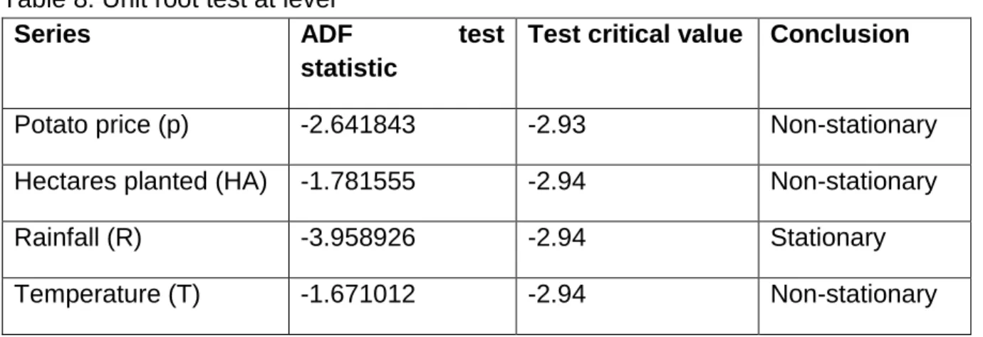
Table 8: Unit root test at level
Series ADF test
statistic
Test critical value Conclusion
Potato price (p) -2.641843 -2.93 Non-stationary
Hectares planted (HA) -1.781555 -2.94 Non-stationary
Rainfall (R) -3.958926 -2.94 Stationary
Temperature (T) -1.671012 -2.94 Non-stationary
Unit root test was performed to tests whether the series is non- stationary and possesses unit root. The Augmented Dickey Fuller statistics value for potato price was – 2.641843, number of hectares planted was -1.781555, temperature was -1.671012 and are greater than critical value ( -2.94) at 5% level, so we do not reject null hypothesis in the above- mentioned series, since time series has a unit root and considered to be non-stationary at level. However, Augmented Dickey Fully statistic value for rainfall level is less than critical value and they possess stationary at level.
29 Table 9: Unit root test at the first differencing
Series ADF test
statistic
Test critical value Conclusion
Potato price (p) -7.204999 -2.94 Stationary
Hectares planted (HA) -8.441654 -2.94 Stationary
Rainfall (R) -18.97811 -2.94 Stationary
Temperature (T) -24.87664 -2.94 Stationary
First differencing was performed. Eviews report that test critical values (- 2.93) at 5% level for all variables were less than their Augmented Dickey Fully values respectively, so the study reject null hypothesis and time series does not have unit root. Therefore, it is stationary. The study confirms that potato price (PP), number of hectares planted (HA) and temperature (T) are non-stationary at level but after first difference, they became stationary whereas rainfall (R) became stationary at level. Nsabimana et al. (2015) who confirmed that all those four series were not stationary at level but they were all stationary after one differencing support the results. Now that all variables are stationary, the study proceeds to the second step, which is to determine cointegration relationship amongst variables. In order to perform cointegration test and VECM model, firstly the study determine the number of optimal lag to be used.
4.4.1 VAR Lag Order Selection
The study has undertaken VAR Lag Order selection process. Various selection criteria results are listed in a table below,
30 Table 10: Lag order selection criteria
Endogenous variables: Number of hectares planted (Ha), Rainfall (R), and Temperature (T).
Lag LogL LR FPE AIC SC HQ
0 -1399.505 NA 8.74e+25 73.92130 74.13677 73.99796
1 -1257.993 238.3358 1.92e+23 67.78910 69.08193 68.24908 2 -1181.598 108.5617 1.38e+22 65.08408 67.45427 65.92738 3 -1157.449 27.96161 1.75e+22 65.12889 68.57644 66.35550 4 -1112.899 39.86078 9.50e+21 64.09993 68.62484 65.70986 5 -1051.638 38.69065 3.24e+21 62.19150 67.79377 64.18474 6 -974.8837 28.27807 1.23e+21 59.46756* 66.14719* 61.84412*
* indicates lag order selected by the criterion
The table 10 indicates information criteria where; AIC (Akaike information criterion), SC (Schwarz criterion) and HQ (Hannan-Quinn information criterion), confirm the lag 6 as the appropriate lag to be used. Therefore, the study proceeds to test for cointegration and VECM using lag 6. Nsabimana et al. (2015), support the results.
4.4.2 Johansen test for cointegration
The study performed Johansen cointegration test using both unrestricted cointegration rank test(Trace) and unrestricted cointegration rank test (Maximum Eigenvalue) to check if there exist relationship between potato price and independent variables. The results are listed in the table below,
Stating null hypothesis as;
𝐻0: There is no cointegration 𝐻1: There exist cointegration