Application of quantitative feedback theory to robust power system stabiliser design.

The result of the QFT design is verified by simulation of the linear and non-linear models representing the power system and also by experimental procedures performed in a laboratory. 0 F.9 S-F\mction of Nonlinear SM File F.lD SM Matrix Initialization File 0 • F .11 SM Matrix Execution File 0 • 0 F.12 Krause Machine Initialization File F .13 Krause Machine Execution File F.14 Initial Conditions Solver File .

List of Tables

Nomenclature

Loop transfer function L(s) Lt armature leakage inductance Ln nominal loop transfer function Lt transmission line inductance. X"q shaft subtransient reactance q Xd shaft synchronous reactance d Xf field leakage reactance Xl armature leakage reactance Xl shaft synchronous reactance q Xt transmission line reactance Xt Xkd d shaft damper leakage reactance Xkq reactance of shaft damper leakage d Xkq shaft damping reactance q.

Introduction

The PSS Problem

INTRODUCTION 2 Since the frequency of oscillation is dependent on the synchronising torque,

Literature Survey

LITERATURE SURVEY
LITERATURE SURVEY 5
LITERATURE SURVEY 16 3. choose a controller for which the nominal closed loop is stable within

Summary

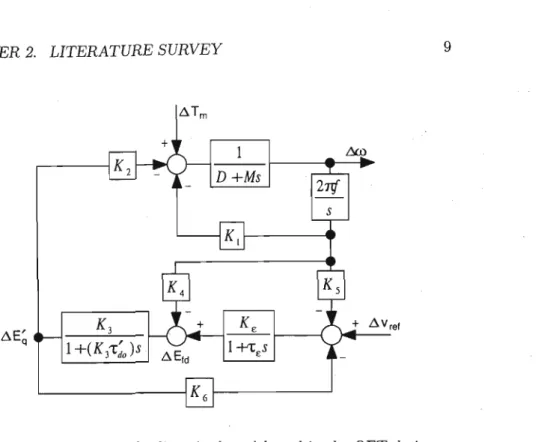
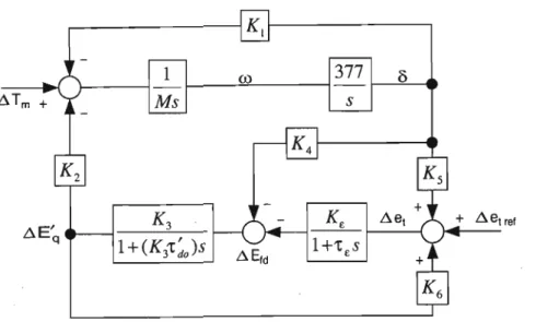
K2 represents the effect of a change in generator flux E~ on torque and increases proportionally [25] as. the stiffness of the ac network increases and 2. The QFTPSS was compared with a PSS state response. The transient response of the QFT design was stable under all operating conditions, while the state feedback controller gave poor transient response.

Figure 2.1: Small signal linear model, including the effect of the voltage regulator-excitation system as used for stability studies.

Mathematical Modelling

MATHEMATICAL MODELLING 18 choosing a particular reference frame is that it will make the resulting com-

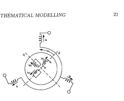
The d-q transformation

MATHEMATICAL MODELLING 19 Assuming the three phase resistance are equal, then R is a non zero, diagonal

Mathematical model of a synchronous gener- ator

MATHEMATICAL MODELLING 21

The 5 electrical equations

MATHEMATICAL MODELLING

The 2 mechanical equations

The transmission line

Summary

The algebraic equations relating the flux linkages to the currents are 1. The derivation of the electric torque for the synchronous machine is complicated and will not be shown here. Tm is positive, in accordance with the sign convention given in Appendix A.I. The two mechanical equations are therefore. 3.40) and including the damping and viscous coefficients, D and K respectively.

Figure 3.1: Physical representation of a synchronous machine showing the 3-phase stator windings and the d-q rotor windings.

Matlab Power System Blockset

Inside the PSB
MATLAB POWER SYSTEM BLOCKSET 29
MATLAB POWER SYSTEM BLOCKSET

Simulating a SMIB

Simulation Results
Summary

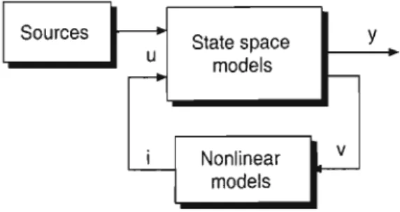
A private Simulink model is built and stored in one of the voltage or current measurement blocks of the main PSB Simulink model. Nonlinear devices are simulated as current sources in the feedback loop of the state space model.

Figure 4.1: Generic private Simulink model built during simulation.

Quantitative Feedback Theory

QUANTITATIVE FEEDBACK THEORY 37 transfer function are observable. Since the transfer function exists,

The Nichols Chart

QUANTITATIVE FEEDBACK THEORY 39
QUANTITATIVE FEEDBACK THEORY

Plant and Loop Transmission Templates

A QFT Example

The QFT Toolbox

QUANTITATIVE FEEDBACK THEORY 53 that ease the design process. One of these is the QFT Toolbox for Matlab [9]

Summary

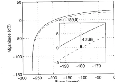
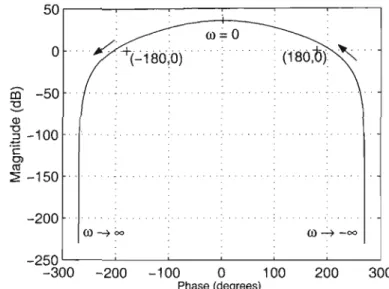
To do this, the Nichols graph must be moved down 4.2 dB. The dotted line shows the Nichols map after it has been moved. At each point, the nominal installation point on the loop transmission template is marked on the Nichols map.

Figure 5.1: A plot on a multi-sheeted Nichols Chart.

The Laboratory Power System

THE LABORATORY POWER SYSTEM 57 relate the theory of power system stabilisers to computer simulation. The

The micro-alternator

The circle is closed when the practical system is used to verify the theory of power system stabilizers. This thesis only describes the transfer function models of the existing power system components in the laboratory. These parameters can be used in the synchronous machine model of Chapter 2 to simulate the micro-alternator.

When using the power system block set, the unit synchronous generator Simulink model must be selected.

THE LABORATORY POWER SYSTEM

Time constant regulator
AVR and Governor

Several measurements were taken of the terminal voltage rise and fall times to a step change in the AVR reference voltage in an attempt to calibrate the TCR. Details on the construction of the TCR and the theory behind it can be found in [33]. The laboratory power system controller is part of the turbine simulator, and will be described in the next section.

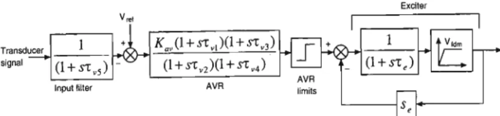
The AVR consists of an input filter to filter the output of the terminal voltage converter, a compensator with hard limits to provide regulation, and a generator amplifier with an upper limit on the field output voltage.

Figure 6.1: Block diagram representation of the laboratory AVR.

THE LABORATORY POWER SYSTEM 60

Turbine simulator

THE LABORATORY POWER SYSTEM Turbine Simulator Values

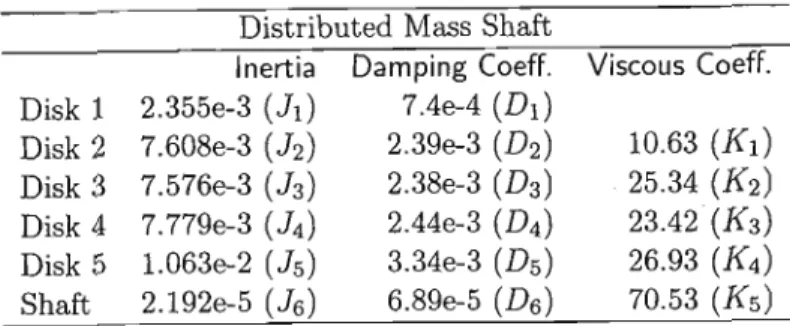
Distributed mass shaft
Transmission line simulator
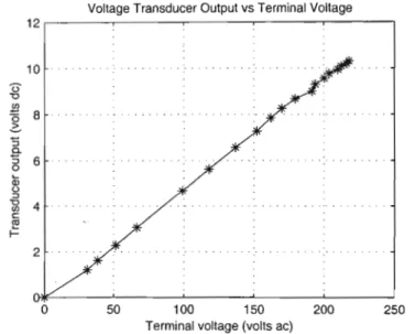
Transducers
Data capture equipment

The problem can be solved if the speed measurement at the generator or the phase delay of the distributed mass axis is measured. The speed deviation transducer is a digital optical circuit that measures the change in the shaft speed of the generator with a shaft encoder. One phase is the reference phase and it is calibrated by aligning the reference coil with the A phase coil of the alternator.

A stroboscope is used to create a stationary image of the rotating protractor attached to the shaft end.

Table 6.4 gives the list of constants for the disks and shaft.

THE LABORATORY POWER SYSTEM 64 to lie within this voltage range. This voltage scaling is done with a gain

Calibration

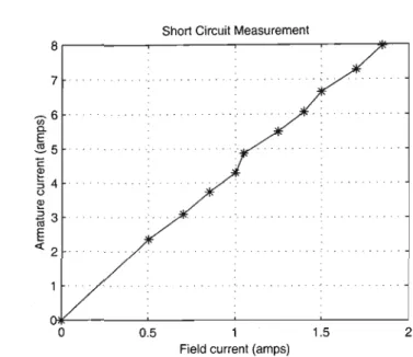
THE LABORATORY POWER SYSTEM Short Circuit Test

Machine tests

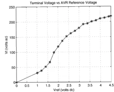
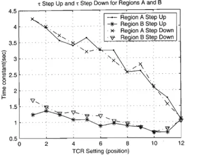
The region of the saturation curve in which the alternator (or any synchronous generator) operates affects the open circuit voltage time constant of the machine. A set of tests was carried out to determine the open circuit voltage time constant for a specific TCR setting at the low end of the saturation curve (denoted as region A in Figure 6.8) and the high end of the saturation curve (denoted region B in Figure 6.8) 6.8 ). The results of the experiment are detailed in Table 6.10 for selected values of the TCR setting.

It can be seen that the time constant for a specific TCR setting varies drastically between the two regions (80Y ac and 200Y ac).

Figure 6.7: Graphical representation of the short circuit results.

THE LABORATORY POWER SYSTEM Open-Circuit Time Constant

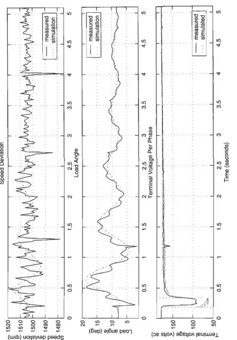
PSB Model vs. Physical Model

Summary

Application of QFT to PSS Design

Linearised Models

APPLICATION OF QFT TO PSS DESIGN 78

APPLICATION OF QFT TO PSS DESIGN

Transmission line

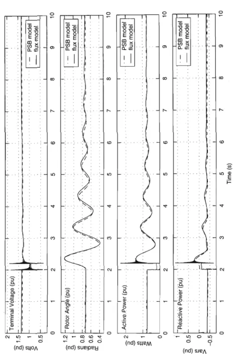
The linearized equations can be used to create a state space model with ABCD matrices available for global processing in Simulink. To test the validity of the linearized equations, it is compared with the nonlinear flow link model given in Appendix F.6 at a specified operating point. We can see that the linear model actually gives the same result as the flux linkage model for small perturbations.

Since the flux linkage model has been verified with the PSB model, it can be said with certainty that the linear model is a linearization of the nonlinear PSB model, at a certain operating point.

APPLICATION OF QFT TO PSS DESIGN 84

Case Study 1: A first-order AVR

The laboratory governor model will be used as well as the laboratory alternator linearized generator model. Since the power system component models are linear time-invariant (LTI) models, the control system toolbox in Matlab can be used to generate an LTI model of the power system. Using the LTI model of the generator connected to an infinite bus via a transmission line as a template, a number of LTI models are generated for different operating points and line reactance.

LTI models are created by calculating the steady state values of the state variables for a given operating point.

APPLICATION OF QFT TO PSS DESIGN 86

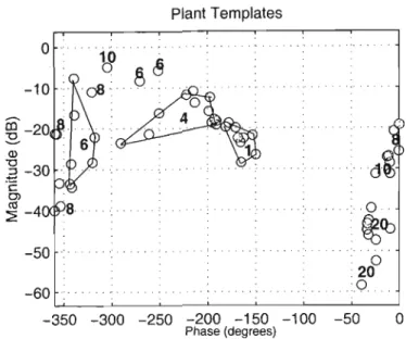
A frequency vector is selected that includes these points, and the plant templates for each frequency are generated. The numbers on the diagram indicate the frequencies at which the plant templates were calculated. The QFT Toolbox is used to calculate the stability limits on the Nichols Chart for all the plant cases.

The label in Figure 7.7 indicates that the output disturbance rejection algorithm was used to calculate the bounds [9].

Figure 7.6: Plant templates for the different power system models.

APPLICATION OF QFT TO PSSDESIGN 92

Case Study 2: Laboratory AVR

APPLICATION OF QFT TO PSS DESIGN 109

Practical implementation
Summary

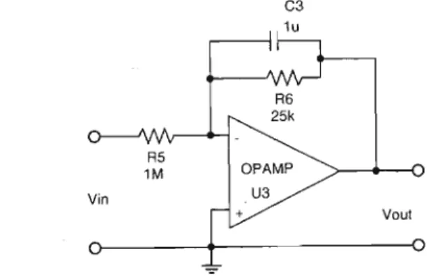
This circuit will be built and used in the power system laboratory to test the QFT design process. The design required the use of analytical linear time-invariant models from which the frequency response had to be calculated. However, what is available, and more importantly what can be measured, is the frequency response.

QFT requires only frequency response data to perform power system stabilizer design, thus making it a powerful tool in this field.

Figure 7.36: Electronic circuit for design equation G 2 (s).

Practical Implementation

PRACTICAL IMPLEMENTATION

Frequency Response Measurements

The relevant power system signals applicable to this experiment are the voltage reference input and the speed signal output. This choice of power system signals is consistent with most of the literature on power system stability [21]. A signal generator is used to superimpose a sinusoidal voltage waveform on the voltage reference input of the AVR.

The reason for choosing 5% is that the overlaid signal does not cause large deviations from the current operating point and thus does not cause non-linear operation of the power system.

PRACTICAL IMPLEMENTATION 115 9. set the signal generator frequency to the required value and the am-

PRACTICAL IMPLEMENTATION 117

Measured PSS Frequency Response

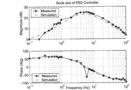
The controller designed in Case Study 2 was tested by measuring its frequency response and comparing it with the simulation bode plot. This was to ensure that the controller was properly built and that the necessary transfer function was realized. A bode plot showing the actual frequency response, along with the predicted frequency response, is shown in Figure 8.4.

It can be seen that the controller is correctly constructed and in fact accurately synthesizes the designed controller transfer function.

Figure 8.4: Bode plot of the designed PSS and simulation PSS.

PRACTICAL IMPLEMENTATION 119

PSS Tests and Results

Operating point 1

PRACTICAL IMPLEMENTATION 122 is a third order Butterworth filter with a -3dB frequency of 5 rad s-1

PRACTICAL IMPLEMENTATION 127 8.3.2 Operating point 2

PRACTICAL IMPLEMENTATION 8.3.3 Operating point 3

PRACTICAL IMPLEMENTATION 137 8.3.4 Operating point 4

PRACTICAL IMPLEMENTATION 141

Summary

The results in this chapter confirmed the use of QFT as a powerful tool in the design of power system stabilizers. Due to the inherent high attenuation of the power system laboratory, the performance criteria were not met. However, not all physical systems allow for frequency response measurements, and a laboratory power supply system is one of them.

This was proven in the laboratory by applying a ground fault to the power system at various operating points.

Conclusions

CONCLUSIONS 144 underlying theory of power systems is still essential, and Chapter 3 provided

Using CAD technology, and understanding how the CAD system models a particular piece of equipment, is critical to generating accurate simulations and predicting the actual behavior of the power system. Once the model of the power system was available for analysis and observation, Chapter 5 introduced the tool that would enable solving the power system stability problem. QFT is a practical control design tool, and Chapter 6 introduced the vehicle on which the designed power system stabilizer would be tested.

The Laboratory Power System is designed to accurately represent an industrial power system many times its rating.

CONCLUSIONS 145 was twofold. Firstly to show the laboratory power system response if the

Bibliography

Ph.d.-afhandling, Department of Electrical and Electronic Engineering, University of Natal, Durban, Sydafrika, december 1991. Ph.d.-afhandling, Department of Electrical and Electronic Engineering, University of Natal, Durban, Sydafrika, oktober 1987. Ph.d.-afhandling, Department of Electrical and Electronic Engineering, University of Natal, Durban, Sydafrika, april 1981.

Master's thesis, Department of Electrical and Electronic Engineering, University of Natal, Durban, South Africa, January 1997.

Appendix A

Machine Theory

I Per Unit System and Sign Convention

Calculating Initial Conditions
Machine Equations in Compact Form

Therefore, in terms of the power flow, the instantaneous power u x i will flow in the circuit if both u andi are positive. The Power System Blockset uses the generator convention, which means that power flows from the circuit if both u and i are positive. Conversion from motor to generator convention is performed by simply negating the signs of the equations.

The machine equations describing a synchronous generator can be written in terms of currents rather than flux.

Figure A.I: Phasor diagram of a synchronous generator.

Appendix B

Laboratory Equipment

Alternator Parameters

Appendix C

Measured PSS Frequency Data

Appendix D

IEEE Excitation and Governor Systems

Excitation system

Steam turbine and governor

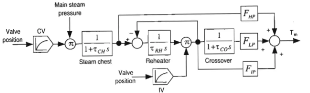
IEEE EXCITATION AND GOVERNOR SYSTEMS 161. is fed to the inlet pipes of the LP turbines via the crossover pipe section. The response of the steam flow to a change in control valve position has a time constant Te H. The reheat contains a significant amount of steam and has a time constant TRH associated with it. Assuming that te is negligible compared to TRH and the control valve characteristic is linear, the simplified transfer function relating control valve position to turbine torque can be written as D.2) The functional block diagram of a mechanical hydraulic regulator system for controlling a steam turbine is shown in Figure D.8.

The speed relay then drives the hydraulic servomotor that controls the valves in the steam turbine.

Figure D.7: Small signal model of the steam turbine suitable for analysis.

Appendix E

Matlab's LTI Toolbox

Creating LTI Models

MIMO systems can be created by specifying H=[Z, P, K], where Z, P, and Kare are P x Mcell arrays of zeros, poles, and gains, respectively. Continuous time models have the form ftx =Ax+Bu andy =ex+Du wherex is the state vector, u is the input vector and y is the output vector. The state space model is created using »sys=ss(A,B,C,D) where A is an x x x state matrix, B is an x x u input matrix, C is a y x x output matrix and D is a y x u throughput matrix.

The AM1MO model is specified by a multidimensional array y x u x N for which the response (y, u,k) is the complex value of the frequency from the input u to the frequency of the output jat frequency (k).

LTI Properties

ZPK models can be specified using the zpk command or using the Laplace variable s. For example, if a model sys is defined, then the input names can be set as. Properties can also be set using the set command, e.g. set(sys,'inputname','temp',outputname,'pressure') A property value can be obtained using the get function, e.g. PropVal=get(sys,'inputname') .

Operations on LTI Models

System characteristics such as rise time, fall time, overshoot and steady state error can be determined from the time response. The impulse command can be used to generate an impulse response, initial can be used to generate an initial state response, and step gives the step response of the system, e.g. step (hiss), impulse (hiss). If the models are stored in an LTI array, the responses of the array models can be plotted by typing bode(LTIArrayName).

Figure E.2: The result of performing multiplication on two LTI models append appends models in a block diagonal configuration, connect forms a state-space model from a block diagonal LTI object for an arbitrary inter-connection matrix

Appendix F

Program Listings

Machine Initialisation file

QFT Design file

Operating Point file

Laboratory System file

N onlinear Operating Point file

Flux Model file