An assessment of abundance trends and biology of langoustines (Metanephrops mozambicus) and pink prawns (Haliporoides triarthrus) from the deep-water trawl fishery off eastern South Africa.

(1)

langoustines (Metanephrops mozambicus) and pink prawns (Haliporoides triarthrus) from the deep-water trawl fishery off eastern South Africa.

BY

JAMES ROBEY

A dissertation submitted in fulfillment of the academic requirements for the degree of

MASTER OF SCIENCE

In the School of Life Sciences, University of KwaZulu-Natal, Durban

affiliated with the

Oceanographic Research Institute

February 2013

(2)

ABSTRACT

Deep-water trawling (>200 m deep) for crustaceans in the South West Indian Ocean (SWIO) yields catches of several species, including prawns (Haliporoides triarthrus, Aristaeomorpha foliacea, Aristeus antennatus and Aristeus virilis), langoustine (Metanephrops mozambicus), spiny lobster (Palinurus delagoae) and geryonid crab (Chaceon macphersoni). Infrequent deep-water trawling takes place off Tanzania, Kenya and Madagascar; however, well- established fisheries operate off Mozambique and South Africa. Regular trawling off South Africa started in the 1970’s, mainly targeting M .mozambicus and H. triarthrus.

Catch and effort data for the South African fishery were regularly recorded in skipper logbooks over a 23 year period (1988 – 2010); this database was obtained from the Department of Agriculture, Forestry and Fisheries (DAFF) in order to assess abundance trends of M. mozambicus and H. triarthrus. Generalized linear models (GLM) were used to quantify the effects of year, month, depth and vessel on catch per unit effort (CPUE). By year, the standardized CPUE of M. mozambicus increased, and three factors (or a combination of them) could explain the trend: reduced effort saturation, improved gear and technology, or an increase in abundance. By month, CPUE peaked in July and was highest between depths of 300 and 399 m. The standardized CPUE of H. triarthrus fluctuated more by year than for M. mozambicus, possibly because it is a shorter-lived and faster growing species. The monthly CPUE peaked in March, and was highest between depths of 400 and 499 m.

Totals of 2 033 M. mozambicus (1 041 males and 992 females) and 5 927 H. triarthrus (2 938 males and 2 989 females) were sampled at sea between December 2010 and March 2012, during quarterly trips on-board a fishing trawler. A GLM framework was used to explore their size composition, sex ratio variability, size at maturity and reproductive cycles. Male and female M. mozambicus size distributions were similar, but varied by month and decreased as depth increased. Female H. triarthrus were significant larger than males; size structure varied by month, but showed no change over depth. The sex ratio of M.

mozambicus favoured males (1 : 0.89), but was close to parity in all months, except November when males predominated. H. triarthrus exhibited parity (1 : 1.002) with no significant variations in sex ratios by month. The proportion of egg-bearing M. mozambicus

(3)

in the population declined between March and August (hatching period) and then increased until December (spawning period). The L50 (length at 50% maturity) of M. mozambicus was estimated to be 49.4 mm carapace length (CL), and the smallest and largest observed egg- bearing females were 33.5 and 68.6 mm, respectively. No reproductively active female H.

triarthrus were recorded during the sampling period.

Growth parameter estimates for M. mozambicus (male and female combined) using Fabens method were K = 0.48 year^-1 and L = 76.4 mm CL. Estimates for the von Bertalanffy growth formula (VBGF) were: K = 0.45 year^-1 and L = 76.4 mm CL. H. triarthrus male and female growth parameter were estimated separately. For males they were K = 0.5 year^-1and L = 46.6 mm CL using Fabens method, and K = 0.76 year^-1 and L = 46.6 mm CL using the VBGF.

For females they were K = 0.3 year^-1 and L = 62.9 mm CL using Fabens method, and K = 0.47 year^-1 and L = 62.9 mm CL using the VBGF.

CL to total weight regressions were calculated for both species; no significant differences were found between male and female M. mozambicus, although H. triarthrus females became larger and heavier than males.

Comparisons with three earlier studies (Berry, 1969; Berry et al., 1975; Tomalin et al., 1997) revealed no major changes in the biology of either species off eastern South Africa. Stocks appear to be stable at current levels of fishing pressure, although some factors are not yet fully understood. Disturbance caused by continual trawling over a spatially limited fishing ground may affect distribution and abundance patterns, especially in M. mozambicus, which was less abundant in the depth range trawled most frequently. The absence of reproductive H. triarthrus in samples suggests that they occur elsewhere, and there is some evidence of a possible spawning migration northwards to Mozambique; this suggests that H. triarthrus is a shared stock between South Africa and Mozambique. The results from this thesis will add to the knowledge of M. mozambicus and H. triarthrus in the SWIO, and provide a basis for developing sustainable management strategies for the deep-water crustacean trawl fishery off eastern South Africa.

(4)

PREFACE

The work described in this thesis/dissertation was carried out at the Oceanographic Research Institute (ORI) which is an affiliated institute of the School of Life Sciences, University of KwaZulu-Natal (UKZN), Durban. Work was conducted from October 2010 to November 2012, under the supervision of Prof. Johan Groeneveld (ORI), Dr. Sean Fennessy (ORI) and Dr. Ursula Scharler (UKZN).

This thesis/dissertation represents original work by the author and has not otherwise been submitted in any form for any degree or diploma to any tertiary institution. Where use has been made of the work of others it is duly acknowledged in the text.

(5)

DECLARATION – PLAGIARISM

I, , declare that:

1. The research reported in this thesis, except where otherwise indicated, is my original research.

2. This thesis has not been submitted for any degree or examination at any other university.

3. This thesis does not contain other persons’ data, pictures, graphs or other information, unless specifically acknowledged as being sourced from other persons.

4. This thesis does not contain other persons' writing, unless specifically acknowledged as being sourced from other researchers. Where other written sources have been quoted, then:

a. Their words have been re-written but the general information attributed to them has been referenced

b. Where their exact words have been used, then their writing has been placed in italics and inside quotation marks, and referenced.

5. This thesis/dissertation does not contain text, graphics or tables copied and pasted from the Internet, unless specifically acknowledged, and the source being detailed in the thesis and in the References sections.

Signed: Date:

James Robey

(6)

REFERENCES ... 84

APPENDIX 1 Permit conditions: KZN prawn trawl fishery ... 101

(7)

ACKNOWLEDGEMENTS

Firstly I would like to thank my supervisors Prof. Johan Groeneveld and Dr. Sean Fennessy for the guidance they have given me, the time spend helping and explaining aspects of this work to me and their commitments and patience while reading through countless drafts of this MSc. For all your help and encouragement I am extremely grateful.

To the South West Indian Ocean Fisheries Project (SWIOPF) for providing the necessary funding and support so that this work was able to be completed. To the Oceanographic Research Institute (ORI) part of the South African Association for Marine Biological Research (SAAMBR) and its entire staff for guidance, assistance and facilities, all of which provided an open and friendly environment to work in.

Thank you to the Department of Agriculture, Forestry and Fisheries (DAFF) and ORI for the collection and provision of an extremely valuable data set without which this project would not have been complete.

A very special thank you to Bernadine Everett, your help in both sorting and analysing data as well as map drawing was invaluable. Thanks to Jorge Santos for assisting with the growth models. And thanks to both of you for your help in explaining the integral workings of GLMs and general comments on data analysis, you were both a great help.

A big thanks to Des Hayes and Chris Wilkinson for the countless days they spent at sea with me, helping collect and process biological samples needed for my work, without you those days would have been even longer. To Knud and Illona Sorenson, from KG Fishing, and the crew of the FV Ocean Spray for allowing me access to the vessel and space to live and work on-board, without your cooperation none of this would have been possible.

To my friends and the guys in the office your general enthusiasm and the good times we shared made the days in front of my computer fly by, thanks.

Tarryn your love, willingness to help, encouragement and support have made my life easy and stress free. Thank you so much, you mean the world to me! Last but not least, to my family (all of you!) without your love and support I’d be lost, thank you so much!

(8)

“Farming as we do it is hunting, and in the sea we act like barbarians. We must plant the sea and herd its animals using the sea as farmers instead of hunters.”

– Jacques-Yves Cousteau

(9)

(10)

* The common names ‘shrimps’ and ‘prawns’ have been used interchangeably throughout the world for both Caridea and Penaeoidea with no consistency and there is much confusion around their use. In Southern Africa the term ‘prawn’ generally refers to larger Natantia (including Penaeoidea) and smaller species are generally called ‘shrimps’ (Holthuis, 1980; Neal and Maris, 1985; de Freitas, 1995). Hereafter the word prawn will be used for all species, unless otherwise stated.

Chapter 1 – INTRODUCTION

1.1 – Background

Decapod crustaceans (including crabs, lobsters, shrimps and prawns*) are highly diverse and abundant throughout the oceans and are vital to marine ecosystems (De Grave et al., 2009).

They are also important species for both commercial and artisanal fisheries worldwide, and are harvested by more nations than almost any other marine organism (King, 1981; Neal &

Maris, 1985; Tully et al., 2003; Ye & Cochrane, 2011). Consequently, many decapod taxa have been extensively studied.

With finfish stocks in decline throughout the world’s oceans (Smith & Addison, 2003) crustacean fisheries are becoming more important. In 2010 the global catch of marine crustaceans amounted to 5.5 million tons (7% of 77.4 million t of all marine catches combined), an increase from 5.3 million t (6% of total catches in 2004) (www.fao.org).

Nevertheless, the annual capture of some groups of crustaceans has shown a decreasing trend over the last few years (Ye & Cochrane, 2011).

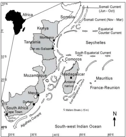
The Western Indian Ocean (WIO) is listed by the Food and Agriculture Organization of the United Nations (FAO) as their fisheries statistical area 51 (Figure 1.1). It has a surface area of approximately 30 million km², of which 6.3% is made up of the continental self, and has a high diversity of oceanographic and fisheries resources. The countries of area 51 include islands and continental states in Africa and Asia. These countries have diverse economies, culture, fishing practices and fisheries management capabilities (De Young, 2006). Fisheries in area 51 are highly important in terms of income and as a major source of animal protein to burgeoning coastal populations, however many fisheries remain relatively unknown and unregulated (van der Elst et al., 2005, 2009; Ye, 2011).

Within area 51, crustaceans account for 9% of the total marine fishery landings. In 2003, total landings of 350 000 t of crustaceans were reported, mainly crab and prawns (van der Elst et al., 2009; Ye 2011). Catches have declined since the 1990’s and recorded catches in 2009 were only half that of the peak catches in the 1980’s and 90’s (Ye, 2011). The cause for

(11)

the decline in crustacean catches, both overall and at species level, is not always clear; in some cases it may be related to overfishing, whereas in others the cause might be environmental change or degradation of habitats (Ye, 2011; Ye & Cochrane, 2011).

Figure 1.1. The Western Indian Ocean, FAO fisheries statistical area 51.

1.2 – South West Indian Ocean (SWIO)

Geographically, the study area covered in this thesis (i.e. eastern coast of South Africa) falls within the South West Indian Ocean (SWIO), which consists of mainly southern hemisphere countries of FAO area 51, along the western edge of the Indian Ocean. The SWIO region includes the exclusive economic zones (EEZ, up to 200 nm from the shore) of nine continental and island nations: Kenya, Tanzania, Mozambique, South Africa, Madagascar, Comoros, Mauritius, Seychelles and France, the latter because of its islands in the region, including La Reunion and Mayotte (Figure 1.2; van der Elst et al., 2009).

The SWIO region is characterised by two major western boundary current systems forming two large marine ecosystems (LME) which encompass coastal areas, the continental shelf

(12)

and the outer margins of the main currents, these LME’s are characterised by distinct bathymetry, hydrography and productivity (Vousden et al., 2008). The Agulhas Current LME stretches from the northern Mozambique Channel to Cape Agulhas; it is dominated by warm and fast-flowing water of the Agulhas Current, which forms part of the anti-cyclonic Indian Ocean gyre. The Somali Current LME extends from the Comoros Islands and northern Madagascar to the Horn of Africa. The Somali Current is dominated by monsoon winds, and flows northwards during the boreal summer (SE monsoon), but its flow is reversed during winter (NE monsoon). Both the Agulhas and Somali LME’s are interactive and influenced by the South Equatorial Current, which is funnelled across the Mascarene Plateau east of Madagascar before diverging north and south to become components of the two LME’s.

These systems influence the climate, weather patterns, sea temperatures, productivity and fisheries of the SWIO region (Lutjeharms, 2006; van der Elst et al., 2009).

Figure 1.2. Countries and major oceanic currents of the SWIO (van der Elst et al., 2009).

The Global Environment Facility (GEF) LME Programme has funded three closely linked projects in a programmatic approach over 5 years (2008 – 2012). These projects were designed to develop and promote scientifically-grounded national and regional fisheries management plans that promote sustainable use of fish resources, while conserving

(13)

ecosystems and biodiversity (Payet & Groeneveld, 2012). The three projects were the Agulhas and Somali Currents LME project (ASCLME, dealing with physical oceanography and productivity), the Western Indian Ocean Land-based impacts on the environment (WIO-Lab, dealing with land-based sources of marine degradation) and the South West Indian Ocean Fisheries Project (SWIOFP, dealing with offshore and shared fisheries resources) (van der Elst et al., 2009). The research in this thesis was funded by SWIOFP, and aimed to provide guidance for the management of deep-water crustacean resources in the SWIO, both at a national level, and at a regional level for shared stocks.

1.3 – Deep-water trawling for crustaceans in the SWIO

The majority of crustaceans captured in the SWIO region are shallow-water (<50 m depth) species, which are easily accessed by artisanal fishers, whereas the deep-water (>200 m depth) stocks are limited to industrialised trawling (van der Elst et al., 2009). Multi-species deep-water crustacean trawl fisheries in the SWIO region catch several species of deep- water prawns (Haliporoides triarthrus, Aristaeomorpha foliacea, Aristeus antennatus and Aristeus virilis) as well as langoustine (Metanephrops mozambicus), spiny lobster (Palinurus delagoae) and geryonid crab (Chaceon macphersoni) at depths of 100 to 600 m (Groeneveld

& Melville-Smith, 1995; Fennessy & Groeneveld, 1997; van der Elst et al., 2009; Groeneveld , 2012). Besides the target crustaceans, non-target species are caught as bycatch (van der Elst et al., 2005); these organisms include many species of teleosts, elasmobranchs and cephalopods which may be retained if their commercial value is high, or discarded if their value is considered too low (Fennessy, 2001). Deep-water crustacean trawl fisheries in the SWIO region are not well known and scientific peer-reviewed publications are scarce (Cunningham & Bodiguel, 2006; Ye & Cochrane, 2011). Data for the majority of countries are minimal and are mainly in the form of survey and stock assessment reports (Groeneveld, 2012).

Deep-water trawling off Madagascar, Tanzania and Kenya is infrequent, due to limited trawling grounds and difficult trawling conditions in comparison to shallow-water trawl fisheries in these regions (Groeneveld, 2012). Several deep-water trawl surveys have taken place in these countries over the past few decades (Crosnier & Jouannic, 1973; Sætersdal et al., 1999; Cunningham & Bodiguel, 2006; Groeneveld, 2012). Mozambique has the largest trawl fishery for deep-water crustaceans in the SWIO region, with trawlable grounds

(14)

covering over 15 000 km² and landings of crustaceans ranging between 1 000 and 3 000 t annually (Silva & Sousa, 1988; Dias et al., 2011). Landings mostly comprise deep-water prawns, with H. triarthrus accounting for 70 to 80% of the catch, and langoustine M.

mozambicus contributing about 10 % (Silva & Sousa, 1988; Dias et al., 2011; Groeneveld, 2012). The neighbouring South African deep-water crustacean trawl fishery is smaller, but fulfils an important niche in the South African fishing industry. Trawling is not permitted in the other SWIO (island) countries.

1.4 – South African deep-water crustacean trawl fishery

Trawling along the eastern coast of South Africa originated from exploratory surveys undertaken as early as the 1920’s which revealed large quantities of the spiny lobster P.

delagoae (Gilchrist, 1922). The spiny lobster was initially targeted and all other species were considered as by-catch, however, in the 1960’s catches of P. delagoae began to decline and the fishery switched to targeting prawns and langoustines (Berry, 1972). Trawling became more regular after 1976, which prompted the development and promulgation of a regulation and control system for the fishery: this was finally implemented in 1988 (Fennessy & Groeneveld, 1997).

Landings of target crustaceans (H. triarthrus, M. mozambicus, P. delagoae and C.

macphersoni) combined ranged between 58 and 215 t/year between 2005 and 2010. During the same period, the average annual landings of M. mozambicus were 36.04 t/year and those of H. triarthrus were 66.34 t/year (Warman, 2011). Trends in effort, catch and catch composition (both crustacean and by-catch, mainly teleosts and elasmobranchs) of this fishery have been described in earlier studies (Groeneveld & Melville-Smith, 1995; Bailey et al., 1997; Fennessy & Groeneveld, 1997; Tomalin et al., 1997; Fennessy, 2001), however, despite the longevity of this fishery and its commercial importance, few biological studies on the target species have been undertaken. Nevertheless, preliminary studies have been done for M. mozambicus (Berry, 1968, 1969; Tomalin et al., 1997) and H. triarthrus (Berry et al., 1975; Tomalin et al., 1997). These two species are the most profitable (Fennessy, 2001) and are captured by deep-water crustacean trawlers within the SWIO region.

(15)

1.5 – Langoustine Metanephrops mozambicus (Macpherson, 1990)

The family Nephropidae supports many fisheries in the world’s oceans (Cobb & Wang, 1985), either as targeted organisms or as a retained by-catch (Bell et al., 2006), and nephropids generally have a high commercial value (Chan & Yu, 1991). The majority of fisheries for Metanephrops species, a sub-family of the Nephropidae, occur in the Indo-West Pacific. A multi-species trawl fishery on the continental slope of north-west Australia catches between 50 and 100 t/year of several Metanephrops species, including M.

australiensis, M. neptunus, M. boschmai and M. velutinus (Holthuis, 1991; Lynch & Garvey, 2005, Bell et al., 2006). The fishery concentrates on muddy substrata at depths of 260 to 500 m. M. challengeri is fished on the continental shelf of New Zealand, on fine sand and muddy bottoms at 140 to 640 m (Wear, 1976; Smith, 1999). Commercial trawlers in the East China Sea capture M. thomsoni on sand and mud bottoms along with several other species (Choi et al., 2008). M. japonicus is fished on sandy mud substrata between depths of 200 and 400 m along the Pacific coast of Japan (Bell et al., 2006; Okamoto, 2008). By far the largest fishery for any nephropid, however, is that for Nephrops norvegicus (Linnaeus, 1758) in the north-east Atlantic and Mediterranean, where total annual landings amount to 50 000 – 60 000 t (Bell et al., 2006). N. norvegicus is caught as a target species and retained as by- catch of multi-species fisheries trawling over muddy substrata in both shallow (20 – 200 m) and deep-water (200 – 800 m) (Chang & Yu, 1991; Graham & Ferro, 2004; Bell et al., 2006).

The above fisheries share many similarities: they target similar depth zones (mainly 200 to 500 m) and substrata (sand, mud), and are multi-species in character. Fisheries for

(16)

Metanephrops species are generally not large, with only a few active vessels, and with limited catches which are sold locally or exported.

The langoustine or African lobster M. mozambicus (Macpherson, 1990) occurs in the Indo- West Pacific region, where it is distributed off eastern Africa between Kenya and eastern South Africa, and off the western coast of Madagascar (Holthuis, 1991). It occurs along the edge of the continental slope on soft muddy substrata at depths of 200 – 750 m, but is most commonly found between 400 and 500 m (Berry, 1968; Berry, 1969; Holthuis, 1991). Prior to 1990, langoustine catches along the east African coast were attributed to M.

andamanicus (Wood-Mason, 1891), a morphologically very similar species from Kenya, the Andaman Sea, the south China Sea and Indonesia (Holthuis, 1991). Macpherson (1990) described M. mozambicus from material collected in Madagascar, and Chan & Yu (1991) identified the main differences between M. mozambicus and M. andamanicus as a more eroded dorsal carina and other sculpturation in M. mozambicus. It remains unclear whether specimens from Tanzania belong to M. andamanicus or M. mozambicus or whether, perhaps, both species occur there (Chan & Yu, 1991). M. mozambicus supports multi- species crustacean trawl fisheries in the SWIO region.

The majority of biological and fisheries research on nephropids have focussed on N.

norvegicus. Many studies have been undertaken and reviews on the biology and fisheries of N. norvegicus are numerous and extensive (see Farmer, 1975; Chapman, 1980; Dow, 1980;

ICES, 1982; Sardá, 1995; Graham & Ferro, 2004; Bell et al., 2006). Studies on Metanephrops species (see Berry, 1968; Berry, 1969; Wear, 1976; Bailey et al., 1997; Tomalin et al., 1997;

Lynch & Garvey, 2005; Choi et al., 2008; Okamoto, 2008) are far less extensive, and many make reference to studies based on N. norvegicus, which include analysis of catch rates, seasonality, growth rates, densities, sex ratios, reproduction and maturity. These studies are helpful for comparative purposes in studies on M. mozambicus within the SWIO region.

Some of the biological characteristics of M. mozambicus along the eastern coast of South Africa were investigated by Berry (1969) and Tomalin et al. (1997). These studies examined morphometry, catch composition, moulting and reproduction. The more recent of the two studies was however undertaken 15 years ago, and since then much more fisheries data has become available. The past 15 years have also seen climate induced changes in marine ecosystems as well as increased anthropogenic impacts on fisheries resources around the

(17)

world (Richardson & Schoeman, 2004; Allison et al., 2009; Brander, 2010). Given these factors, a re-examination of the biology and fishery targeting M. mozambicus off eastern South Africa was considered to be justified.

1.6 – Pink prawn Haliporoides triarthrus (Stebbing, 1914)

Prawns are divided into two superfamilies; 1) Penaeoidea, which form the basis of many artisanal and trawl fisheries in tropical and sub-tropical regions and 2) Caridea, which are more widely distributed, but less commonly fished (Holthuis, 1980; King, 1981; Neal & Maris, 1985). Of the Penaeoidea, the family Solenoceridae includes the genus Haliporoides which comprises three species of medium to large prawns important to commercial fisheries (Holthuis, 1980). H. diomedeae is distributed in the eastern Pacific from Panama to Chile where it is caught by multi-species deep-water crustacean trawl fisheries (Holthuis, 1980;

Arana et al., 2003; Parraga et al., 2010). H. sibogae and H. triarthrus are distributed along the continental shelves or slopes of the Indo-West Pacific, where they also support multi- species deep-water crustacean trawl fisheries (Holthuis, 1980; de Freitas, 1985).

H. sibogae has been reported off Madagascar, the Malay Archipelago and New Zealand (Holthuis, 1980), but it is more common in the waters of Australia, Japan and in the East China Sea (Baelde, 1991; Kosuge & Horikawa, 1997; Ohtomi & Matsuoka, 1998). The Australian fishery is small, but well established and stable, and is located off the south-east coast (Baelde, 1992). This species is targeted by trawlers on muddy grounds at depths of 270 to 850 m (mostly 400 to 500 m) and annual production ranges between 300 and 350 t at

(18)

a catch rate of around 80 to 100 kg/trawl hour (Baelde, 1991, 1992, 1994). H. sibogae off Japan and in the East China Sea has been targeted by commercial bottom trawlers since the 1960’s, with annual landings ranging from 350 to 500 t (Kosuge & Horikawa, 1997; Ohtomi &

Matsuoka, 1998). These landings have decreased since the 1980’s, stimulating increased research (Ohtomi & Matsuoka, 1998).

Multi-species trawl fisheries off the east coast of Africa catch H. triarthrus, along with other deep-water crustaceans, on soft muddy bottoms along the continental slope, most commonly between 360 and 460 m depth (Holthuis, 1980; de Freitas, 1985). H. triarthrus is commercially fished off Mozambique and South Africa and potential deep-water trawl fisheries have been found by trawl surveys off Madagascar and Tanzania (Groeneveld, 2012).

However, in the latter two countries the trawl grounds are limited and fishing conditions are difficult due to strong currents and bottom topography; fishing companies have therefore focussed mainly on the extensive shallow-water fishing grounds (Groeneveld, 2012). The Mozambique deep-water crustacean fishery is the largest in the SWIO region, with annual landings ranging between 1 500 and 2 700 t of crustaceans, of which H. triarthrus contributes 70 to 90% (Torstensen, 1989; Torstensen & Pacule, 1992), whereas the South African fishery lands <100 t of this species per year.

Many fisheries surveys of the deep-water trawl grounds of Mozambique have taken place over the past few decades (see Brinca et al., 1983; Sobrino et al., 2007a; Sobrino et al., 2007;

Dias et al., 1999, 2008, 2009, 2011; Dias & Caramelo, 2005, 2007) and the data have, inter alia, been used to assess the abundance and biology of H. triarthrus (see also Torstensen, 1989; Torstensen & Pacule, 1992). However, fewer studies of this species are available from South Africa (Berry et al., 1975; de Freitas, 1985; Tomalin et al., 1997), despite its importance to the local fishing industry, its trans-boundary distribution pattern, and the high likelihood that H. triarthrus is a shared resource between South Africa and Mozambique.

The research in this thesis was justified due to the large time gaps between studies of H.

triarthrus off South Africa as well as the possible impacts of climate change on fisheries over the last few decades (Allison et al., 2009).

(19)

1.5 – Aims of this study

Studies of animal communities inhabiting the continental shelf and slope are an important aspect of marine ecology, particularly where they have a significant commercial value (Abelló et al., 1988). The effects of trawling on the environment may include altered habitats, reduced biodiversity, and changed population demographics (i.e. abundance, size and sex distributions) of affected species, which may result in reduced productivity, and impact on the sustainability of a fishery (Tuck et al., 1998; Hansson et al., 2000;

Schratzberger et al., 2002; Bell et al., 2006; Zhou et al., 2010).

With this in mind, the aims of the present study were to use fisheries and biological data collected during sampling trips at sea on-board commercial trawlers off the east coast of South Africa, to investigate langoustine M. mozambicus and pink prawn H. triarthrus populations so as to determine: (a) distribution patterns on the fishing grounds; (b) population demographic structure (sex and size structure); (c) reproductive biology (size at maturity, breeding season); and d) somatic growth rates. A long-term database (1988 – 2010) comprising logbook information of catches and effort per trawl recorded by the skippers of fishing vessels, and stored by the national Department of Agriculture, Forestry and Fisheries (DAFF), was analysed to determine trends in abundance of the two species over the past two decades.

The results of the present study were compared to the findings of Berry (1969), Berry et al.

(1975), de Freitas (1985), Bailey et al. (1997) and Tomalin et al. (1997) on M. mozambicus and H. triarthrus off eastern South Africa. The outcome of this study was used as the basis for developing fisheries management strategies based on best-available information.

(20)

Chapter 2 – MATERIALS and METHODS

2.1 – Study area and gear

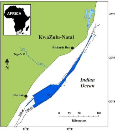
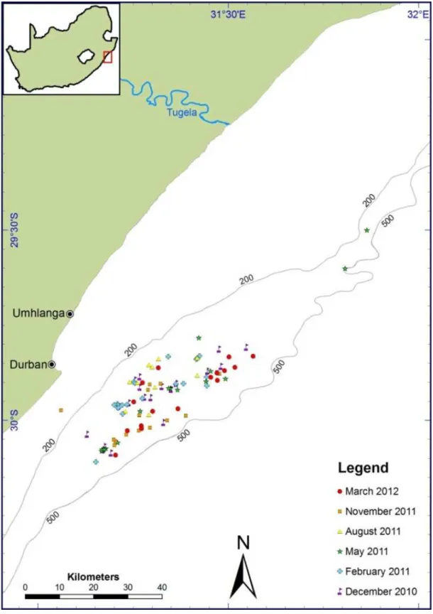
Samples were collected from bottom trawls undertaken on the trawling grounds off the eastern coast of South Africa, between 28 and 31° S (Figure 2.1). Between these latitudes, in the Natal Bight, the continental shelf is at its widest, extending up to 50 km offshore (Lutjeharms et al., 1989), and providing a relatively large trawlable area of about 1 750 km² between 100 and 600 m (mostly 300 – 500 m) (Berry, 1969; Groeneveld & Melville-Smith, 1995; Fennessy & Groeneveld, 1997). At these depths the substratum ranges from areas of hardened sediment to mud, mainly consisting of foraminiferous remains (Berry, 1969; Berry et al., 1975). The Agulhas Current core meanders close to the continental shelf edge in this region (Lutjeharms, 2006), and generally flows in a south westerly direction, with speeds of up to 3 knots being common (Berry, 1969; Lutjeharms, 2006). Berry (1969) found the average bottom temperatures on the trawl grounds to range between 9 and 12 °C, however recent measurements suggest that it is somewhat cooler, between 8 and 10 °C at 500 m depth (L. Guastella, University of Cape Town, unpubl. data).

Figure 2.1. Deep-water trawling grounds off eastern South Africa.

(21)

All sampling trips were undertaken during normal fishing operations on board a commercial deep-water trawler operating from Durban harbour. The FV Ocean Spray is a stern trawler (LOA of 35 m; GRT of 282 t; 800 hp engine) using a single otter trawl with ‘V’ shaped doors, weighing 630 kg each. The nylon trawl net was attached directly to the doors, and had a 60 mm stretched mesh size over the body, wings and cod end (Figure 2.2). The net had a foot rope length of 50 m with 45 m of chain attached, and a head rope length of 40 m. The effective height between the foot and head rope, while fishing, was approximately 1.5 m.

Figure 2.2. Generalised otter trawl net.

2.2 – Sampling procedure

Six quarterly sampling trips were undertaken between December 2010 and March 2012.

Trawl data including set and haul time, GPS position (start of trawl), depth range and trawl speed were recorded for each drag. Once the net was emptied onto the deck, a random sample was collected by shovelling 10 to 20 kg of the catch into a plastic crate. The sample was weighed to the nearest kg and the targeted crustacean component was separated from the rest of the crate contents and reweighed. An estimate of the total weight of M.

mozambicus and H. triarthrus caught per trawl, based on the number of boxes of packed by the crew, was obtained from the skipper.

(22)

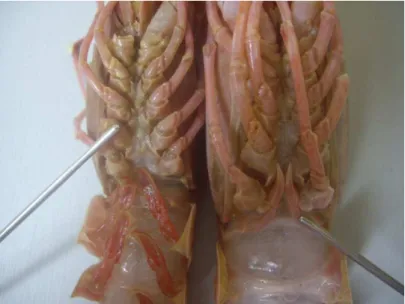
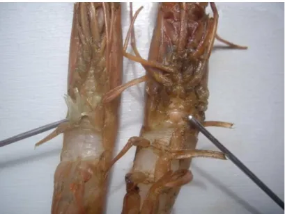
Biological data were collected from all individuals of M. mozambicus and H. triarthrus in the subsample. M. mozambicus individuals were sexed based on the position of the external genital openings (Figure 2.3); females have paired oviducts which open on the coxae of the third pereiopods and the vas deferens of males opens through a slightly raised aperture on the coxae of the fifth pereiopods (Berry, 1969; Farmer, 1975). Female H. triarthrus were identified by the presence of the thelycum, between the 3^rd and 5^th pereiopods, and males were identified by the petasma, found on the first pleopod (de Freitas, 1985) (Figure 2.4).

Carapace lengths (CL ± 0.1 mm) for both species were measured as the distance between the base of the inner eye socket and the posterior margin of the carapace, using vernier callipers. The shell condition was recorded as being either ‘hard’ or ‘soft’.

Figure 2.3. Positions of female (left) and male (right) M. mozambicus genital openings.

Figure 2.4. Positions of the male petasma (left) and female thelycum (right) of H. triarthrus.

(23)

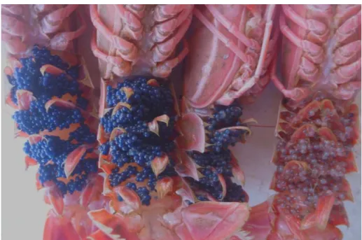
The numbers of egg-bearing M. mozambicus females in samples were recorded, and eggs carried on the abdomen of females were staged as follows (Berry, 1969) (Figure 2.5):

1. Freshly spawned = Bright royal blue/no embryo development 2. Early embryo development = Dark blue-purplish/embryo visible as thin tissue 3. Well-formed embryo = Dark purple to pink/appendages just visible 4. About to hatch = Red/fully formed, eyes of larvae visible

Male reproductive organs could not be staged macroscopically and due to time and space constraints on board the vessel the maturity status of M. mozambicus males was not recorded.

Figure 2.5. Four development stages of M. mozambicus eggs, stage 1 on the left through to stage 4 on the right.

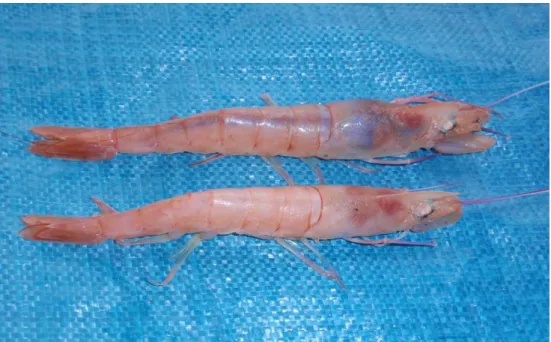
The numbers of reproductively active H. triarthrus females were recorded and ovarian development was staged as follows (Berry et al., 1975):

1. Inactive / immature = Thin, clear or faintly pink/not swollen 2. Active = Pink to red/slightly swollen

3. Ripe = Blue-grey/swollen

4. Spent = Grey-yellow/flaccid

(24)

The staging of H. triarthrus female ovaries was conducted macroscopically, as the ovaries were visible through the dorsal exoskeleton (Figure 2.6). However, male reproductive organs were not macroscopically visible and they were therefore not staged.

Figure 2.6. Colour change of female H. triarthrus ovaries, visible as a bright blue mass in the top prawn (ripe), and as a faint thin line in the bottom prawn (inactive/immature) (Photo by S. Fennessy, Oceanographic Research Institute).

In addition to the onboard sampling, boxes of M. mozambicus and H. triarthrus packed by the crew in three size classes (large, medium and small, 2 kg of each) were purchased directly from the vessel during months in which sampling at sea did not take place. The CL, sex, egg developmental stage (M. mozambicus), ovarian stage (H. triarthrus) and shell condition of these specimens were determined in the same way as during field trips and in addition individual weights were recorded to the nearest gram in the laboratory. These samples were used solely in the determination of the length-weight relationships for both species.

(25)

2.3 – Data analysis

CPUE

Information on catches and effort was obtained from the Department of Agriculture, Forestry and Fisheries (DAFF) for the entire commercial trawling fleet, as recorded in logbooks by skippers as part of permit conditions (DAFF 2012; Appendix 1), between 1988 and 2010. The data were cleaned by removing anomalous records, in which the trawl localities, depth, date or catches were clearly inaccurate. The dataset contained a large number of zero catches per trawl of M. mozambicus and H. triarthrus; this was considered to reflect the multispecies nature of the fishery, in which other crustacean species (i.e. spiny lobster or geryonid crab) were targeted on occasion. Nevertheless, the zero catches contain information on the distribution patterns of the two species being investigated, and therefore they were included in the analysis.

The catch (packed weight per trawl) and effort (trawl hours) were used to determine the nominal catch per unit effort (CPUE, in kg/hour) for both species. The nominal data provide a coarse indication of CPUE and abundance, however this index may be biased by gear- effects, changes in catchability, and spatio-temporal variation within the stock (Kimura, 1981; Salthaug & Godo, 2001; Sbrana et al., 2003).

The effects of year, month, depth and vessel on CPUE were first quantified using a generalised linear model (GLM), and thereafter a standardised index of abundance was calculated to correct for the influences of the variables shown above. The statistical software package R version 2.14.0 (R Development Core Team, 2011) was used to fit the GLMs.

One of the main challenges of modelling catch rates (or CPUE) in fisheries is that these data often have many zero catches per unit of effort (i.e. per trawl or per trap set) and these must, in some way, be included in the analyses. Currently, the most popular way for dealing with large numbers of zero catches is to use the delta method, in which the zero and non- zero records are analysed separately (Maunder & Punt, 2004). This involves fitting two sub- models to the data (Lo et al., 1992; Maunder & Punt, 2004; Shono, 2008; Carlson et al., 2012). The first sub-model assigns a value of zero or one based on the respective absence or

(26)

presence of a species, and assumes a binomial error distribution (2.1) with a Logit link function, and quantifies the probability of occurrence (or of capture) of the species.

The binomial probability density function as described by Haddon (2001) is:

| , = _! ^! _! 1 − (2.1)

where: is the probability of an event, , occurring in, , trials.

In the second sub-model, only the positive catches are modelled assuming either a gamma, log-normal or Poisson distribution. Preliminary tests showed that the relationship between the logarithms of the mean and variance of the CPUEs (positive values) were close to two, showing that the data were highly dispersed, and consequently a gamma model (2.2) with a Log link function was selected to fit the second sub-model.

The gamma distribution function as described by Haddon (2001) is:

| , = _{!" #} $ (2.2)

where: is the value of variate , is the shape parameter and Γ( ) is the Gamma function for parameter .

Explanatory variables tested included year, month, depth and vessel (Table 2.1). Latitude and longitude were excluded as explanatory variables from this model, because the majority of trawling takes place within a small well defined area of the fishing grounds, causing an unbalanced spread of the data over the entire fishing ground as well as uncertainty in trawl locality data prior to 2000, when a coarse grid method of positioning was in use. The standardised CPUEs were computed by multiplying the probability of catch (from the binomial model) with the conditional catch (from the gamma model) which were in turn obtained from the coefficients of each model. For both sub-models the year 1988, month August, depth 400 m and the most active vessel in the fleet were used as reference points, as these were the most frequent and representative observations of these factors. The standardised and nominal CPUEs were plotted for each explanatory variable.

(27)

Size

A GLM framework, using R software, was further used to analyse size, sex ratios and maturity of M. mozambicus and H. triarthrus. Data for these analyses were obtained from the onboard sampling as detailed above. A Gaussian error distribution (2.3) with a Log link function was selected to model the size data, for both species. The explanatory variables year, month, depth and sex were tested and those not significant in explaining deviations from the mean were omitted from the final selected model (Table 2.1). The outcome from the standardised size models was plotted for each explanatory variable.

The Gaussian distribution function as described by Haddon (2001) is:

%|&, ' = _*√,-⁾ .^/ ^{0 1 2}²³² ⁴ (2.3)

where: %|&, ' is the likelihood of any individual observation %, given μ population mean and σ population standard deviation.

Sex ratio

A binomial error distribution (2.1) with a Logit link function was selected to model sex ratios of both species. The explanatory variables tested included year, month, depth and CL. The only significant variable explaining the sex ratio of M. mozambicus was month and for H.

triarthrus month and CL were significant (Table 2.1). The outcomes from the standardised models were plotted as a probability of capturing a male for both species.

Maturity

The presence of eggs on female M. mozambicus was used as the indicator of maturity and only females were therefore considered in the model. Month, depth and CL were significant explanatory variables in determining maturation of M. mozambicus. These data were modelled using a binomial error distribution (2.1) with a Logit link function (Table 2.1). The outcomes from the standardised maturity model were plotted, as a probability of capturing a mature female by month and depth, and as a logistic curve to determine maturity.

Carapace lengths at which 25% (L25), 50% (L50) and 75% (L75) of females reached maturity were estimated using a logistic ogive (2.4) and numeric values were determined by back calculation, using the inverse Logit.

(28)

The logistic ogive of any number (α) is given by the inverse-logit as follows:

5678 ⁾ 9 = _):⁾ _; = _):^;_; (2.4)

No reproductively active H. triarthrus females were recorded in any samples and subsequently no analyses could be performed.

Model and explanatory variable selection

All final GLMs were selected based on a stepwise approach, which involved modeling all possible combinations of error structures, link functions and explanatory variables (Table 2.1). Explanatory variables were selected based on factors that were likely to influence the catchability of each species. Those model combinations with the smallest AIC values and best fits to the data (based on visual assessments of residual plots) were selected for the final model (Akaike, 1974; Maunder & Punt, 2004). An assumption of the models including the variable ‘vessel’ was that vessel was considered a fixed effect, thus allowing models of CPUEs of each vessel to be calculated in relation to a reference vessel. Maunder & Punt (2004) showed that interactions in the models between variables (e.g. year and vessel) are common and can be significant, but are difficult to account for. These interactions were ignored in this study, an approach used by Vignaux (1994) (Maunder & Punt, 2004), however it should be noted that abundance indexes may be biased in the approach. The decision as to the choice of categorical or continuous variables, in the case of length and depth, was based on the AIC values as well as residual plots of each model run. However, Maunder &

Punt (2004) recommend that continuous variables be treated as categorical, if it simplifies the model and better explains the data. Where appropriate in the analysis these considerations were taken into account.

(29)

Table 2.1. Factors retained in the final GLMs for M. mozambicus and H. triarthrus. The delta method was used to model CPUEs. Year, month and depth were treated as categorical variables and length as a continuous variable. The Akaike information criterion (AIC) was used in the selection of final models.

Growth

Growth estimates were calculated from data obtained from the onboard sampling as detailed above. Descriptions of growth patterns in crustaceans frequently rely on analysis of length-frequency distributions (Farmer, 1973; Hillis, 1979; Gulland & Rosenberg, 1992).

With this approach, the first step was to assess if there were differences between the onboard-sampled monthly distributions of CL for males and females using Pearson’s χ² tests of independence (Townend, 2002). Length-frequency distributions were pooled, as samples were collected from a small area, narrow depth range and from a commercially operating vessel, thereby disallowing a carefully planned random stratified approach to sampling.

These were plotted and visually analysed to assess the presence and number of modes, which were interpreted as cohorts or age classes, and for signs of progression of these cohorts. After a preliminary assessment of the modes, more exact estimates of their proportions, mean lengths, standard deviations and standard errors were calculated using Solver, the optimization tool available in MS Excel. Software developed in MS Excel mimicked the program MIX (Macdonald & Pitcher, 1979; Macdonald & Green, 1988) and assisted in the separation of mixtures of normal or gamma distributed modes. Either the likelihood of the multinomial distribution, or simple least squares of the totals could be used as fitting criteria (Haddon, 2001).

Model Species Error Link Explanatory Variables AIC

CPUE M. mozambicus Binomial Logit Year + month + depth + vessel 43027 M. mozambicus Gamma Log Year + month + depth + vessel 231985

H. triarthrus Binomial Logit Year + month + depth + vessel 29079 H. triarthrus Gamma Log Year + month + depth + vessel 320583

Size M. mozambicus Gaussian Log Month + depth 14848

H. triarthrus Gaussian Log Month + depth 33770

Sex ratio M. mozambicus Binomial Logit Month 2804.8

H. triarthrus Binomial Logit Month + length 7863.7 Maturity * M. mozambicus Binomial Logit Month + depth + length 758.06

* Calculated only for M. mozambicus females

(30)

In order to discriminate between modes in the length frequencies three major assumptions were made in the fitting and characterization of the modes: (1) that the length observations within each mode were normally distributed (2) that increments between mean lengths of the same cohort decreased with size (or time) and (3) that standard deviations remained relatively constant. This ensured that the model fitted to the obvious modes correctly, by setting constraints on the mean, proportion and standard deviation of the modes.

The best fitting parameters of the different modes (proportion, mean and standard deviation) were then searched by minimization of least squares using Solver in MS Excel.

Although many modes were identified for M. mozambicus, discrimination within the oldest and youngest modes proved difficult, and thus only two cohorts were used in the analysis.

Those two best represented the data, as they had the highest number of modes, and could be traced over the entire study period. Male and female H. triarthrus showed only one cohort each, which could be more easily traced over time.

The von Bertalanffy growth function (VBGF) was fitted to the length data of M. mozambicus for sexes combined and individually by sex for H. triarthrus, using two methods. The first method was the traditional VBGF (2.5) with the following equation:

_< = ₌>1 − . ? < <@ A (2.5)

where: _< is the length at time t, ₌ is the mean asymptotic length, K is the growth coefficient and t0 is the theoretical age at the start of growth.

This method required an explicit definition of the age or time of birth and operated with temporal growth. The age or birth date was assigned to the initial cohort, which was determined based on the proposed reproductive cycles and biological characteristics of both species (see Berry, 1969; Berry et al., 1975; de Freitas, 1985) and then the age of each cohort was traced over time.

(31)

The second method used was Fabens (1965) method (2.6) with the following equation:

∆ = _{< : )}− _< = ₌− _< ∙ 1 − . ^?.∆< (2.6)

where: ∆ is the change in size increments, _< and _<:) are the mean cohort lengths measured at ∆8 time periods apart, ₌ is the mean asymptotic length and E^the growth coefficient.

Fabens method, which is based on a transformation of the VBGF, does not require a known age, and circumvents this requirement by dealing with size increments instead. In the present study the units of the parameters were millimetres and years. During the fitting process it was often difficult to obtain convergence to a reasonable asymptote, and the maximum CL recorded was set to be 95% of L= for both species, a method described by Pauly (1980). The two cohorts selected from the M. mozambicus data followed similar growth trajectories and a single VBGF was fitted to the combined data, as the Pearson’s χ² test indicated no significant differences between the monthly length frequencies. However, the VBGF were fitted to male and female H. triarthrus separately as this test indicated there were significant differences in the monthly length frequencies (see results). The two versions of the VBGF were fitted using Solver, by means of non-linear least squares assuming a normal error structure of the observations.

Length weight relationships

Data collected from samples bought monthly (as described above) were used to determine the relationship between CL and whole weight (WW) by fitting linear models using a least- squares algorithm in Microsoft Excel for both species. Data were non-linear and consequently the data were log-transformed, and relationships compared by sex using linear models.

Length weight curves (2.7) were drawn using the exponential equation:

G = 9 ∙ ^H

(2.7) where: G is the whole weight and the carapace length, of an individual and α and β are

parameters of the model.

(32)

Chapter 3 – RESULTS

3.1 – General

A total of 49 991 deep-water crustacean trawls were analysed, as captured onto a database by DAFF, from logbooks returned by skippers over a 23 year period. The total landed catch of both species during this time was 4177.67 t with an average of 181.64 ± 53.43 t/year. The average trawl duration over this period was 4.24 ± 1.23 hours and the average trawl depth was 399.35 ± 82.07 m.

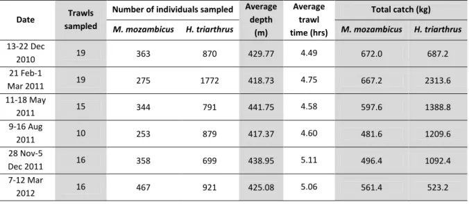
The trawl and biological data collected during the 6 on-board sampling trips undertaken for this thesis are summarised below (Table 3.1), and the locations of the sampled trawls are shown in Figure 3.1.

Table 3.1. Summary of the trawl and biological data collected during on-board sampling trips.

Date Trawls sampled

Number of individuals sampled Average depth

(m)

Average trawl time (hrs)

Total catch (kg)

M. mozambicus H. triarthrus M. mozambicus H. triarthrus 13-22 Dec

2010 19 363 870 429.77 4.49 672.0 687.2

21 Feb-1

Mar 2011 19 275 1772 418.73 4.75 667.2 2313.6

11-18 May

2011 15 344 791 441.75 4.58 597.6 1388.8

9-16 Aug

2011 10 253 879 417.37 4.60 481.6 1209.6

28 Nov-5

Dec 2011 16 358 699 438.95 5.11 496.4 1092.4

7-12 Mar

2012 16 467 921 425.08 5.06 561.4 523.2

(33)

Figure 3.1. Start positions of trawls sampled during on-board sampling trips.

(34)

Nominal effort and landings

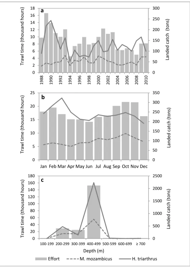
Nominal fishing effort (total time trawled) over the 23 year period peaked in 1989 at over 16 600 trawling hours (Figure 3.2a), but during 1994 it declined to only 27% of the peak effort, mainly because a major fishing company did not fish during that year. Fishing effort recovered between 1995 and 2003. In 2004 fishing effort declined to almost half that of the 2001 peak of 12 300 trawl hours, and remained at this low level up to 2008, whereafter it recovered. The landed mass of M. mozambicus increased between 1988 and 1993, remained relatively constant up to 2000, and then declined up to 2008. A recovery in landings was reported for 2009 and 2010. Landed catches of H. triarthrus peaked in 1990 at just over 240 t, whereafter they declined. A low of 52 t was reported in 1994 (when there were fewer vessels in the fishery), but overall a gradually increasing trend was observed between 1994 and 2009, when catches amounted to 190 t.

By month, fishing effort was highest in spring and summer (September to February) with a decrease in December and was lowest over the autumn and winter months, between April and August (Figure 3.2b). Monthly aggregated catches of M. mozambicus steadily increased from January to a peak of 140 t in October, thereafter declining towards November and December. The monthly trend in catches of H. triarthrus showed a peak in March (335 t) followed by a gradual decline to a low by December (196 t).

Little time was dedicated to trawling shallower than 200 m and deeper than 500 m, with the majority of the effort concentrated in the 200 to 499 m depth range, and over 80% of this effort occurred between 400 and 499 m (Figure 3.2c). The landed catches of both M.

mozambicus and H. triarthrus increased with depth to peak between 400 and 499 m depth, whereafter they declined sharply beyond 500 m.

(35)

3.2 – Metanephrops mozambicus

CPUE

M. mozambicus was one of the targeted species and was present in 79.95% of all trawls made between 1988 and 2010. The total catch over the 23 year period was 1 231.45 t, at an average of 53.54 ± 18.97 t/year. The average nominal CPUE was 5.9 ± 8.89 kg/hour.

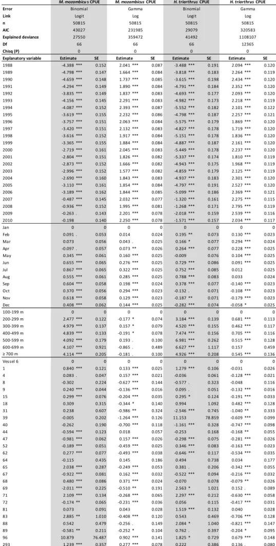
Year, month, depth and vessel were all significant explanatory variables in the first sub- model (presence/absence, binomial model) of the CPUE for M. mozambicus (Table 3.2). The probability of capturing M. mozambicus increased between 1989 and 2007, and thereafter it remained high up to 2010. By month, the highest probability of capturing M. mozambicus was July; the probability decreased up to December and remained low from January to April, but increased again in May and June. By depth, the probability of capturing M. mozambicus was lowest between 100 and 299 m, and peaked between 300 and 399 m. As depth increased beyond 400 m the probability began to decline, and this decrease correlated with a marked increase in trawling effort in the 400 to 500 m depth stratum.

There was no identifiable trend in the probability of capture by vessel, with some vessels having significantly greater probabilities than others; factors affecting this may include vessel power, gear configuration, the total time each vessel operated in the fishery and experience level of the skipper. The same explanatory variables were also significant in the second sub-model, the gamma model for positive catches (Table 3.2), and the product of these two sub-models were used to generate the standardised CPUE.

(36)

Figure 3.2. Nominal fishing effort (hours trawled) and landed catch of H. triarthrus and M.

mozambicus for the fishing fleet by a) year, b) month and c) depth.

0 50 100 150 200 250 300

0 2 4 6 8 10 12 14 16 18

1988 1990 1992 1994 1996 1998 2000 2002 2004 2006 2008 2010 Landed catch (tons)

Trawl time (thousand hours)

a

0 50 100 150 200 250 300 350

0 5 10 15 20 25

Jan Feb Mar Apr May Jun Jul Aug Sep Oct Nov Dec

Landed catch (tons)

b

0 500 1000 1500 2000 2500

0 20 40 60 80 100 120 140 160 180

100-199 200-299 300-399 400-499 500-599 600-699 ≥ 700

Landed catch (tons)

Depth (m)

c

Effort M. mozambicus H. triarthrus

(37)

Table 3.2. Coefficients (±SE) of parameters tested in the final GLMs describing CPUE of M.

mozambicus and H. triarthrus. p < 0.0001 indicated by ***, p < 0.001 **, p <

0.01* and p < 0.05 ^. .

Error Link n AIC

Explained deviance Df

Chisq (P)

Explanatory variable SE SE SE SE

1988 -4.388 *** 0.152 2.041 *** 0.087 -3.488 *** 0.191 2.094 *** 0.120

1989 -4.798 *** 0.147 1.664 *** 0.084 -3.818 *** 0.183 2.264 *** 0.119

1990 -4.659 *** 0.148 1.737 *** 0.085 -3.615 *** 0.198 2.434 *** 0.120

1991 -4.294 *** 0.149 1.890 *** 0.084 -4.791 *** 0.184 2.352 *** 0.120

1992 -3.835 *** 0.149 1.837 *** 0.083 -4.693 *** 0.177 2.093 *** 0.120

1993 -4.156 *** 0.145 2.291 *** 0.083 -4.982 *** 0.173 2.218 *** 0.119

1994 -4.087 *** 0.152 2.393 *** 0.087 -5.552 *** 0.182 2.101 *** 0.122

1995 -3.619 *** 0.155 2.232 *** 0.086 -4.798 *** 0.187 2.257 *** 0.121

1996 -3.757 *** 0.151 2.063 *** 0.084 -5.575 *** 0.179 1.869 *** 0.120

1997 -3.420 *** 0.151 2.132 *** 0.083 -4.827 *** 0.178 1.719 *** 0.120

1998 -3.616 *** 0.152 1.917 *** 0.084 -5.151 *** 0.178 1.836 *** 0.120

1999 -3.365 *** 0.155 1.884 *** 0.084 -4.887 *** 0.187 2.161 *** 0.120

2000 -2.719 *** 0.161 2.045 *** 0.083 -5.449 *** 0.178 2.237 *** 0.120

2001 -2.804 *** 0.151 1.826 *** 0.082 -5.337 *** 0.174 1.810 *** 0.119

2002 -2.873 *** 0.152 1.666 *** 0.082 -4.943 *** 0.175 1.968 *** 0.119

2003 -2.996 *** 0.152 1.577 *** 0.082 -4.859 *** 0.179 2.125 *** 0.119

2004 -2.690 *** 0.160 1.843 *** 0.083 -4.937 *** 0.183 2.301 *** 0.120

2005 -3.110 *** 0.161 1.854 *** 0.084 -4.797 *** 0.191 2.527 *** 0.120

2006 -3.189 *** 0.162 1.844 *** 0.085 -5.099 *** 0.186 2.369 *** 0.121

2007 -0.487 *** 0.145 2.032 *** 0.077 -1.320 *** 0.161 2.275 *** 0.115

2008 -0.936 *** 0.152 1.995 *** 0.081 -1.268 *** 0.171 2.795 *** 0.119

2009 -0.263 . 0.143 2.201 *** 0.078 -2.018 *** 0.159 2.539 *** 0.116

2010 -0.198 0.140 2.250 *** 0.078 -1.571 *** 0.157 2.034 *** 0.117

Jan 0 0 0 0 0 0 0 0

Feb 0.091 . 0.053 0.014 0.024 0.195 ** 0.073 0.130 *** 0.023

Mar 0.073 0.056 0.043 . 0.025 0.166 * 0.077 0.294 *** 0.024

Apr -0.097 . 0.057 0.073 ** 0.026 0.264 *** 0.077 0.228 *** 0.025

May 0.345 *** 0.061 0.160 *** 0.025 -0.009 0.076 0.104 ***