Cooling trends are observed in the southern part of the Benguela Upwelling System in Australian summer and autumn. Coastal upwelling refers to the upwelling that takes place along the coasts of the continents.
Literature review
- Study area
- Mean atmospheric circulation
- Oceanic circulation: Surface and Subsurface currents
- Variability in the Benguela upwelling: interannual variability, trends and decadal
- Interannual variability of the Benguela Upwelling System
- Trends and Decadal Variability
The Benguela Upwelling System is influenced by the South Atlantic Current (Veitch et al., 2010) that brings the South Central Atlantic Water (SACW) and the East Central Atlantic Water (ESACW) towards the BUS. Recently, using a coupled ocean–atmosphere model, Vizy et al. 2018) found a negative trend in mixed layer temperatures in the Northern Benguela Upwelling.

Thesis objectives
Furthermore, there are possible links between the rainfall of the region and the western and southern coast of Southern Africa (Wolski et al., 2021).
Thesis outline
Data
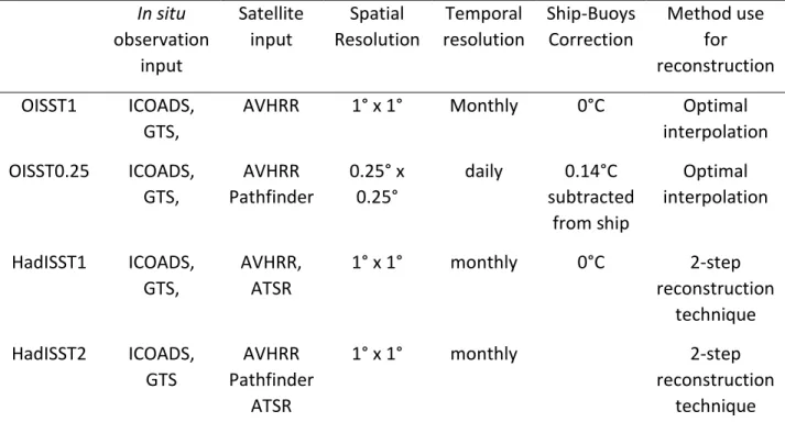
- Gridded observational oceanic data
- Weekly Optimum Interpolation Sea Surface Temperature (OISST)
- Daily OISST
- Hadley SST version 1
- Hadley SST version 2 (HadISST2)
- Extended Reconstructed Sea Surface Temperature version 5 (ERSST5)
- AVHRR Pathfinder version 5.3
- Climate indices
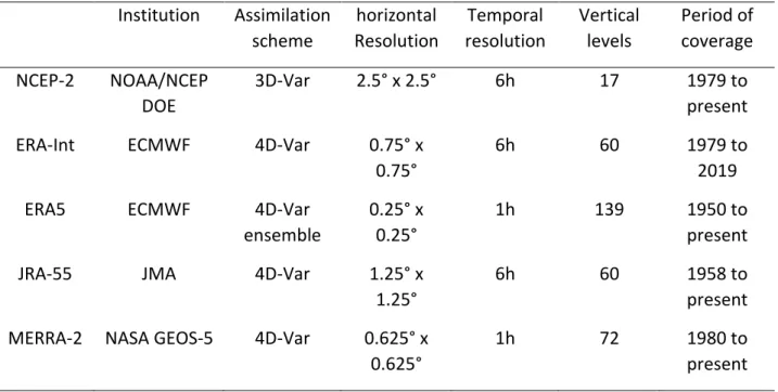
- Atmospheric Reanalysis datasets
- NCEP-DOE reanalysis II
- Era-Interim
- ERA5
- Japanese 55-year reanalysis JRA-55
- MERRA-2
- Ocean model outputs
- Tropical Atlantic Simulation (TATLT025) using NEMO 3.6
- Global ocean simulation using the ocean-ice components of the NorESM
Pathfinder was also used by Blamey et al. 2015) to create their SST trend in the Benguela Rise System. The Japan 55-year reanalysis (JRA-55) is the second global reanalysis of the Japanese atmosphere produced by the Japan Meteorological Agency (JMA) (Kobayashi et al., 2015).

Methods
- Linear least square regression fit (linear trend)
- Linear trend
- Statistical significance test for the trend (Student’s t-test)
- Monthly anomalies and normalization
- Filtering procedure
- dSST derived from net surface heat fluxes
- Wavelet analysis
- Wavelet power spectrum
- Wavelet coherence
- Composite and bootstrap
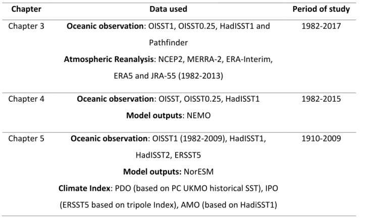
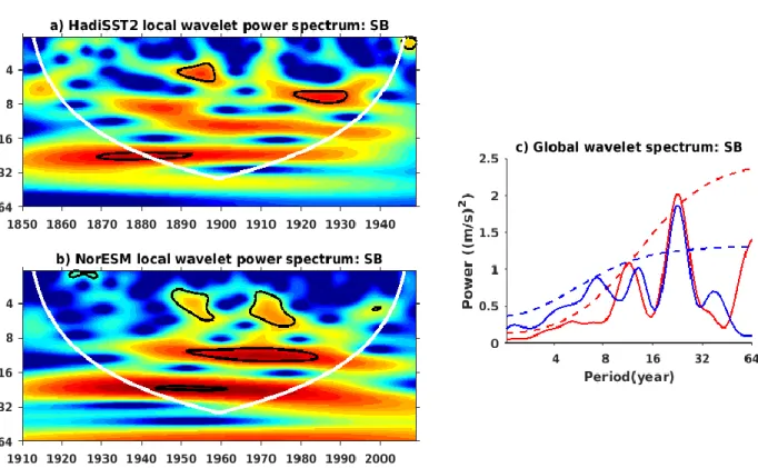
Finally, I use HadISST1, HadISST2, ERSST5, and NorESM to investigate decadal variability in the Benguela Upwelling System over the past 110 years. To investigate a possible decadal variability in the Benguela growth system over the past 100 years (chapter 5), monthly anomalies or normalized anomaly data have been removed.
Introduction
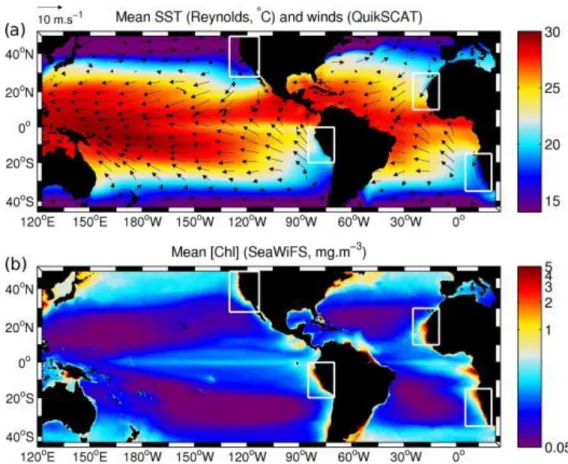
These problems may arise from SST retrieval techniques, the spatial resolution of the data, and/or the potentially strong SST biases observed by some satellites in the Benguela upwelling system. In this study, I use a comprehensive comparative approach based on multiple SST datasets and a reanalyzed wind dataset to compute a trend analysis in SST and wind speed in the Benguela upwelling system and to test the possible existence of decadal variability. To do this, I first compare SST data and reanalysed wind data in the Benguela Upwelling System by analyzing their long-term mean and annual cycles.
Long-term mean and seasonality in the Benguela Upwelling System
Long-term means of SST
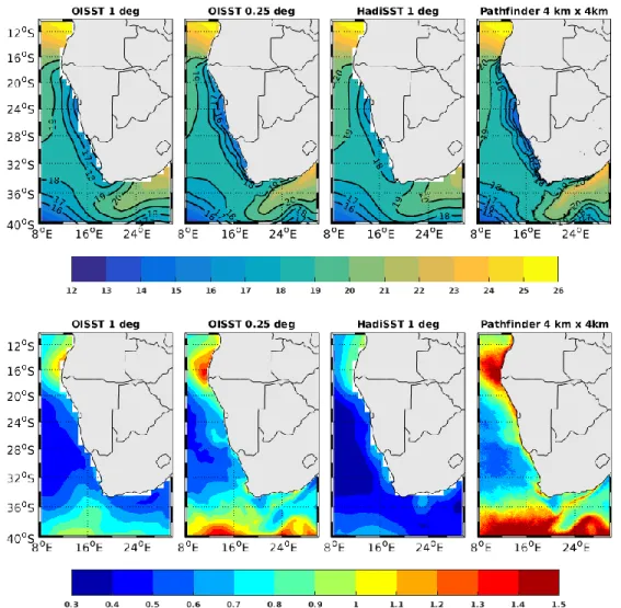
The annual standard deviation of the monthly anomalies of the SST data sets (Figure 3.1, lower panels), reveals a spatial difference in SST variability along the east coast of the South Atlantic. SST in the Benguela Upwelling System and SASH show less variability compared to SST in the two coastal boundaries of the Benguela upwelling, the ABF and the Agulhas region. In the Benguela Upwelling System, the standard deviation is less than 0.7°C with the SST datasets except Pathfinder, where the standard deviation is about 0.9°C close to the coast.
Annual cycle of SST
In the Agulhas Current region, especially the Agulhas Retroflexion Zone, the SST standard deviation is ~0.9°C for OISST1 and greater than 1.3°C for OISST0.25 and Pathfinder. Comparison between datasets (Figure 3.3) reveals that in ABF and the Benguela Upwelling System, HadISST1 has the warmest SST throughout the year, while OISST0.25 and Pathfinder have the coldest SST. In the ABF (Figure 3.3 top left panel), the maximum SST varies between 20 and 24 °C, depending on the data sets, and is observed in March.

Annual cycle of wind
- Long-term means of wind
- Annual cycle of meridional wind
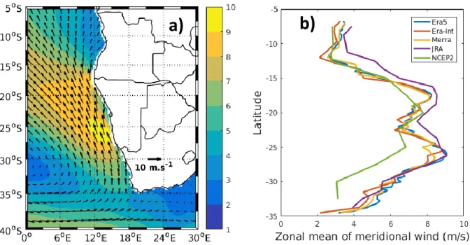
As mentioned in the previous section, weak equatorward meridional winds ranging from 2 to 4 m.s-1 are observed north of the ABF and in Southern Benguela. A maximum is observed in ABF and the second is observed in CB with values varying between 8 and 9 m.s-1. I also note that NCEP2 shows the weakest wind in the annual cycle in the CB and SB.
Trends in SST
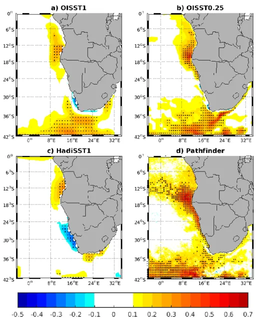
Overall trends
Disagreement in SST trends occurs among the datasets especially along the coast in the Benguela Upwelling system. A statistically significant cooling trend, ranging from 0.2 to 0.4°C, is observed in the Central and Southern Benguela using HadISST1 data set while a warming trend is observed almost everywhere in the Benguela Upwelling System with the Pathfinder data set (Figure 3.6 c and d). A cooling trend of less magnitude and spatial extent than HadISST1 is observed in the south of the Benguela using OISST1 and OISST0.25 (Figure 3.6 a and b).
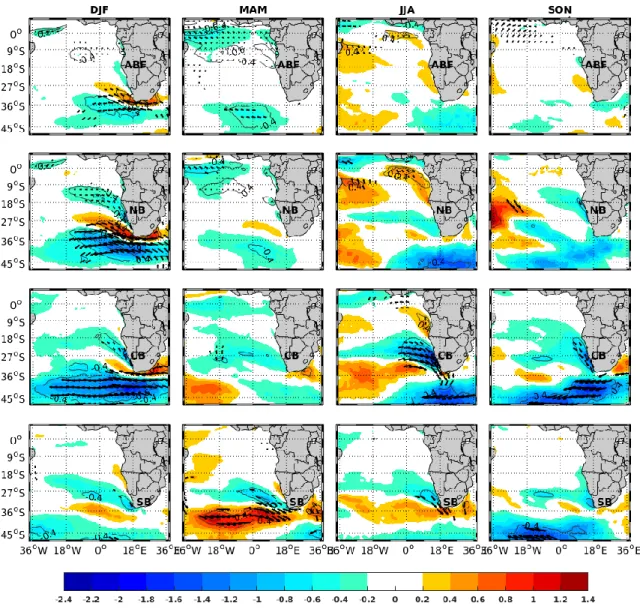
Seasonal trends
Except for HadISST1, the datasets also agree that a significant warming trend is observed in the open ocean and the Agulhas Current south of 33°N. The regional-scale trend difference for products (OISST1, OISST0.25, HadISST1, Pathfinder) based on the same AVHRR space instrument is a cause for concern. Cross lines indicate statistically significant values at the 95% level using Student's t test based on linear regression.
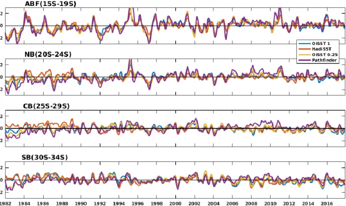
Comparison of monthly timeseries of SST anomalies in the four domains to understand
Correlations between SST anomalies between datasets in ABF are greater than 0.8 except for the correlation between HadISST1 and Pathfinder which is 0.76 (Table 3.1). Pearson correlations are respectively and 0.5 between HadISST1 and OISST1, HadISST1 and OISST0.25 and between HadISST1 and Pathfinder. Analysis of similar trends over the period Figure 3.9) shows a fairly good agreement between OISST1, HadISST1 and OISST0.25.
Trends in wind
Overall trends in wind speed
The positive trends observed along and near the coast of Namibia and South Africa's west coast are not statistically significant. This may be due to a problem in the reanalysis datasets calculated with nearshore model outputs. In fact, most of the statically significant values are not near the coast, but offshore and near the Angolan coastal zone.
Seasonal trends in wind speed
These negative wind speed trends are more pronounced and statistically significant in the austral winter (JJASO) period. In the Benguela upwelling system, I observe that in the austral summer (DJFMA), statistically significant positive trends up to 0.7 m.s-1 are observed in the Southern Benguela in all datasets, consistent with the SST cooling. However, the positive trends are only statistically significant in the North Benguela in all datasets except MERRA-2.

Regression and Correlation between wind and SST
The influence of the SASH wind is more pronounced in the NB compared to the ABF area, which is logical. These results suggest that in the austral summer a poleward shift of the SASH reduces the southerly and southeasterly winds in the ABF and NB, which in turn increases the SST in these regions. These results confirm that a poleward shift of the SASH increases the southerly and southeasterly winds in Southern Benguela, which cool the SST at.
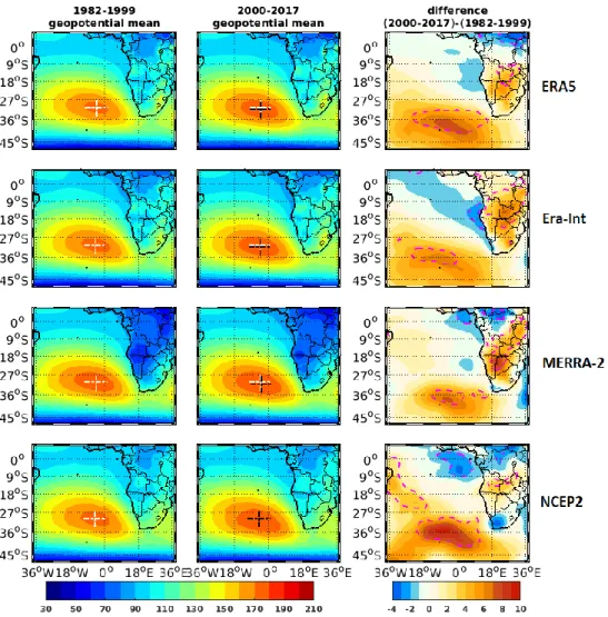
Intensification and poleward displacement of SASH
In addition, the core of SASH in the period 2000-2017 has expanded to the south in all datasets. Positive trends in SASH center size are statistically significant at the 95% level in all data sets. Positive trends in the size of the SASH center are observed throughout the year in all data sets (Figure 3.17).
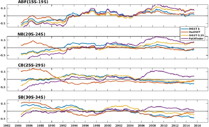
Decadal variability of SST in the Benguela Upwelling System
However, the variability differs from one domain to another and from one data set to another, especially in the Benguela eddy system. In the SB domain (Figure 3.22), all datasets except HadISST1 show significantly increased variance from 1992 to 1997. This is observed in the ABF cushion zone with all datasets, in the CB domain with HadISST1 and Pathfinder, and in the SB- region for OISST0.25, HadISST1 and Pathfinder.
Discussion and summary
Cooling trends are observed in the southern part of the ascending Benguela system and are present throughout the austral summer (Figure 3.9). Finally, I found that the warming or cooling trends in the Benguela upwelling system are not linear. In the next chapter, I will explore the origin of the warming trend in the ABF and northern Benguela.
Introduction
Maximum wind speed is 8 m/s in the south and minimum wind speed is 3 m/s just north of the ABF. A tropical Atlantic configuration of the OGCM NEMO model ((Madec et al., 2017), hereafter NEMO) is used for this study. Finally, I will highlight the role of the Angola dome in the austral summer warming of the Angola-Namibia region.
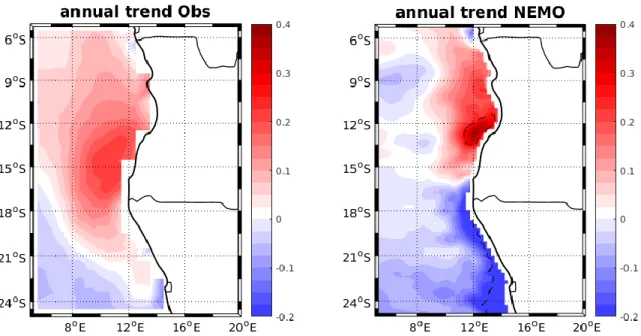
Comparison of SST trend in NEMO with observations in the ABF
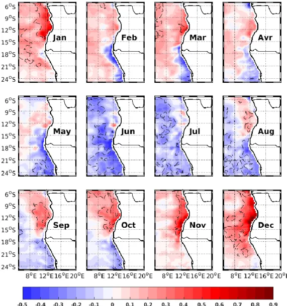
There is also a cooling trend south of 18oS in the observations from April to October, while there is a warming trend in the rest of the year. A cooling trend is also statistically significant south of 22oS from July to September in the observations. On a seasonal scale, the model represents the Australian summer warming trend and the winter cooling trend in the ABF and northern Namibia well, but the model overestimates the cooling trend.
Upper-ocean heat budget analysis in the mixed layer
This cooling is associated with horizontal advection of heat and is very strong along the Namibian coast, offsetting the net surface heating term. Indeed, the zonal advection of heat, except in the open sea of the Angolan and some parts along the Angolan coast between 11°S and 13°S, cools the ocean. The meridional advection of heat also heats the sea along the coast of northern Namibia (north of 23°S) and cools the open sea off the Namibian coast.
Upper-ocean heat contribution in seasonal SST trend
Positive trends in dSST are also observed in the Angolan open ocean in early Australian summer (November, December, January). In addition, in Australian winter, dSST shows positive trends in the ABF coastal zone, while SST shows negative trends. Relatively small positive depth trends of mixed layers down to 1.5 m per decade are observed in early summer (October to December) off the northern Angolan coast to about 9°S in late summer (January–February) in the region's open ocean found in Angola.
Role of Horizontal currents in seasonal SST trend
Climatology of horizontal current
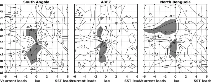
The poleward trend observed in May–June decreases the equatorward one observed during this period, while the equatorward one in July–August increases the equatorward one during the period. There is a 1-month lag between the poleward trend observed in currents and the warming trend in SST. In ABF, except in December and May, negative statistically significant lag correlations of up to −0.7 are found when the meridional current anomalies lead SST anomalies with a 1-month lag.
Role of vertical currents
Climatology of vertical current
Statistically significant negative correlations of up to -0.7 are observed when the meridional current anomalies lead the SST anomalies by 1 month. However, from January to March there are significant lag correlations with lags of up to 5 months when the meridional current anomalies lead to the SST anomalies. The upward trend in the Angolan sector is weak compared to what is happening in the Namibian sector.
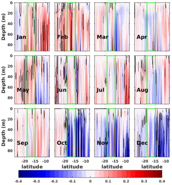
Seasonal trends of vertical currents
The green box indicates the latitude of the ABF and the black dotted lines indicate statistically significant values at a 95% confidence level using the Student's test based on linear regression.
Role of the Angolan Dome in summer warming of the Angola-Namibia coast
This Angola dome is associated with the cyclonic curve of the South Equatorial Undercurrent, which feeds the Angola Current (Peterson and Stramma, 1991; Wacongne and Piton, 1992). Furthermore, the presence of the Angola Dome from September to April coincides with the poleward Angola Current (Figure 4.9). The cooler the underground temperature in the Angola Dome region (Figure 4.14), the stronger the Angola Current (Figure 4.9).
Discussion and conclusion
However, the cooling and warming patterns in the NEMO outputs are consistent with the trend in GODAS, ORA-S4, and CRCM shown in Fig. 2 in the study by Vizy et al. This result contrasts with that of Vizy and Cook (2016) who suggested that the warming trend in Australian SST along the coast of Angola and Namibia is associated with a net downwelling increase. I also note that the warming trend observed along the Angolan and Namibian coasts reaches 100 m depth during the early austral summer, while the rest of the year is only observed in the upper mixed layer.
Introduction
To our knowledge, there are few works on decadal SST variability in the Benguela Upwelling System. For example, Venegas et al. 1997) in their study found interdecadal fluctuations of approximately 14–16 years in the South Atlantic basin. Signals were detected in the Western Cape winter rainfall, the South Benguela growing region and the summer rainfall for the rest of southern Africa.
Validation of the model NorESM
- Comparison of long-term mean SST in NorESM with Observations
- Wavelet analysis
- Reconstruction of timeseries of the dominant timescale with lower frequencies
- Correlation between SB SST and local meridional wind
- Correlation between SB SST and SB Qnet
On a quasi-decadal time scale (9-14 years), SB SST and SB meridional wind show coherence values greater than 0.7;. The anticorrelation between SB SST and SB meridional wind on a time scale of 9-14 years is also observed in the period 1910-1920. As in the previous section, the figure shows good agreement between SB SST and SB Qnet on the dominant SB SST time scales: interannual time scale (2–8 years), quasidecadal (9–14 years), and interdecadal time scale (19–26 years).
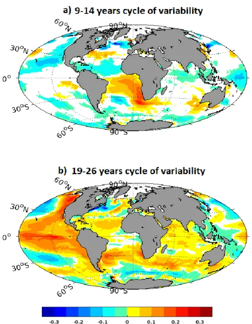
SB SST multiscale relationship with global SSTs
SB SST and global SST anomalies
Positive SB SST anomalies are also associated with cold anomalies in the tropical North Atlantic (0–30°N) and SST in the California upwelling system. In contrast to the quasidecadal scale of variability, on the interdecadal scale, positive SB SST anomalies are associated with warm SST anomalies (> 0.2°C) in the tropical Pacific, surrounded by a horseshoe pattern of opposite sign. Positive SB SST anomalies are also associated with warm SST anomalies in the subtropical Atlantic and Indian Ocean.
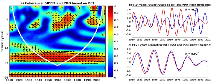
Correlation between Southern Benguela SST with climate modes
The correlation between the reconstructed PDO index and SB SST on the interdecadal scale is about R = 0.92 (Figure 5.9c and table 5.1). The correlation between the reconstructed PDO index and SB SST is about R = -0.23 (Figure 5.9c) on the near-decadal time scale. Higher coherence between the SB SST and the IPO index is observed on the interannual time scale (2–8 years) and on the interdecadal time scale.
Discussion and conclusion
The Benguela upwelling system, one of the four main coastal upwelling regions in the world ocean, is of great importance. Rouault (2015), Ecosystem change in southern Benguela and underlying processes, Journal of Marine Systems, 144, 9-29. Mohrholz (2012), Response of Benguela upwelling systems to spatial variations in wind stress, Continental Shelf Research, 45, 65-77.