In this study, the Spectral Quasilinearization Method (SQLM) coupled to finite difference and the Bivariate Spectral Quasilinearization Method (BSQLM) in solving second-order nonlinear evolution partial differential equations are compared. However, there has been no study comparing these methods in solving partial differential equations of second-order nonlinear evolution.
Background of the Problem
This thesis discusses the comparison of the spectral quasilinearization method combined with finite difference and the bivariate spectral quasilinearization method in solving second-order nonlinear evolution partial differential equations. It is still crucial to carry out more research in finding the solution of partial differential equations for nonlinear evolution with the aim of improving the accuracy.
Review of Nonlinear Partial Differential Equations
After years of research, scientists therefore approximate the solution of the system of partial differential equations using numerical discretization techniques to some function values at certain distinct points, which are called grid points or grid points. To overcome such problems, the spectral method has taken over and has become the most popular method in the last two decades due to the accuracy and efficiency it brings to the calculation.
Review of Spectral Methods
Another method that has been used which is based on spectral methods is the spectral relaxation method. Another method based on spectral methods is the Local Spectral Linearization approach used by Motsa et al.
Aims and Research Objectives
Modeling error: These errors arise due to the difference between the real problem and the mathematical model. According to David in [25], there are two main reasons for this, namely: (i) the magnitude of the change in time is usually limited by explicit stability conditions, and the stability of the time integration requires that the time difference errors be negligible, (ii) many problems include multiple spatial coordinates, so that potential efficiency in representing the spatial disparity of the dependent variables is important to the overall performance of the method.
Problem Statement
Significance of the Study
Plan of the Dissertation
Third, the Burgers-Fisher equation is considered as another example of the nonlinear evolution equation. The application of second-order Burgers-Fisher nonlinear evolution equations describes numerous processes in science and biology, e.g.
Properties of Numerical Methods
Accuracy and Consistency
Convergence error: It is the difference between the numerical solution and the exact solutions of the given equations. Such errors are essentially algorithmic errors and can predict the magnitude of the error that will occur in the method.
Convergence and Stability
SQLM uses the finite difference method for time derivatives and the spectral method for spatial derivatives. It is then important to note that finite difference methods are local methods while spectral methods are global methods.
Describing the Spectral Quasilinearisation Method with Finite Difference 23
For the purpose of this study, our focus is on PDEs, which are discussed in the next section. The spectral method should provide more accurate results than the other methods traditionally used in the past, for example the finite difference method [25]. The origin of the method lies in the theory of dynamic programming and was first initiated by Bellman and Kabala in 1965 [16].
In equation (3.6) the index 0,1 and 2 represent the derivatives ofu, u0andu00 with respect to when the sum is expanded. 71]. The basic idea of the collocation method is to approximate the unknown solution of u(x, t) over the entire domain by a higher order Lagrangian polynomial at the given collocation points. The partial derivatives in the variable x are approximated by the derivatives of the Lagrangian polynomial.
Space derivatives are approximated by differentiation matrices and time derivatives are approximated by finite difference methods, which are discussed in the next section.
Time Descritisation
Explicit Spectral Quasilinearisation Method (ESQLM)
The scheme represented by equation (3.20) is called fully explicit as it calculates un+1i+1 from the quantities known at times. The model is presented in Matrix form as shown by equation (3.20) which will be solved using Matlab.
Implicit Spectral Quasilinearisation Method (ISQLM)
Crank-Nicolson Spectral Quasilinearisation Method (CN-SQLM) 33
Since the bivariate Lagrange interpolation is used, one of the variables is kept constant while the other varies. The most crucial step in the implementation of the solution is the evaluation of the time derivative at the grid points ts for s = 0,1,2,. Using the Lagrange polynomial in equation (4.5), the values of the time derivatives at collocation points (xr, ts) are calculated for s= 0,1,2,.
This chapter discusses the approximation of the solutions of nonlinear evolution equations using spectral quasilinearization method coupled with finite differences in time and the bivariate spectral quasilinearization method, which uses spectral method in both time and space derivatives. It will demonstrate the applications of the methods by solving second-order nonlinear evolution equations. To illustrate the convergence and accuracy of the schemes, the infinity norm error is considered.
The approximate solution at each time level and the corresponding exact solution are used to determine the level of accuracy of the methods.
Numerical Experiments
Burgers Equation
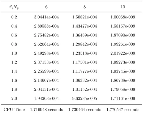
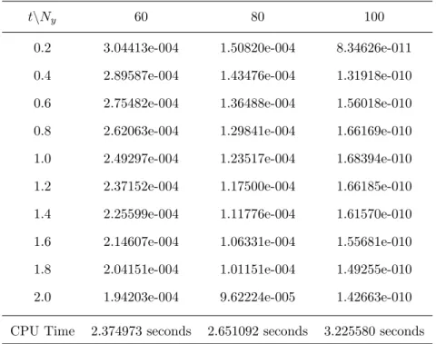
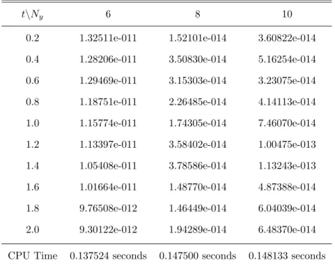
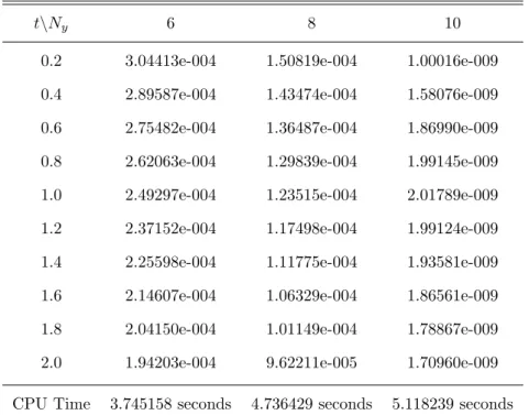
For the purpose of comparing the numerical methods, the following Burgers equation is considered. The infinite norm errors for SQLM and BSQLM are shown in Tables 5.1–5.4 with the corresponding central processing (CPU) times in seconds. The same case for the Burgers equation is also solved by the bivariate spectral quasilinearization method.
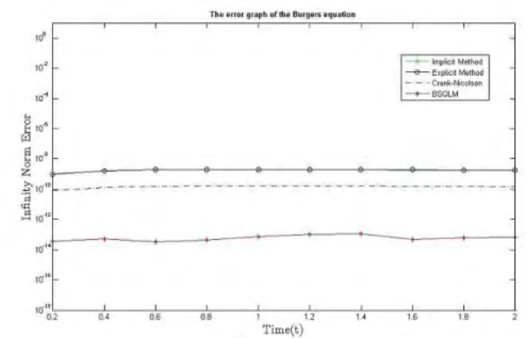
It can be seen that CN-SQLM and BSQLM produce a small infinite norm error with the smallest in BSQLM. The results in Tables 5.1 - 5.4 indicate that BSQLM is much better than SQLM in solving the Burgers equation. It was observed that the BSQLM gives a very accurate solution with an infinite norm error of up to 10−14, CN-SQLM with an infinite norm error of up to 10−11, while the ESQLM and ISQLM have errors of 10−9.
For both the SQLM and BSQLM methods, the infinity rate error shown in the tables is consistent with the plot.
Fisher’s Equation
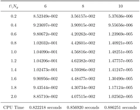
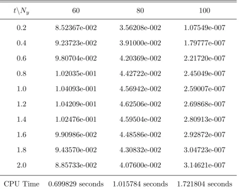
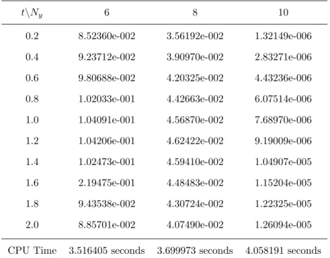
The infinity standard errors are presented in Tables 5.5 - 5.8 for both methods and their corresponding CPU times. The infinity norm error decreased as the number of collocation points increased more significantly compared to SQLM. Fisher's equation was solved in this subsection, and the infinity standard errors are shown in Tables 5.5–5.7 for ISQLM, ESQLM, and CN-SQLM.
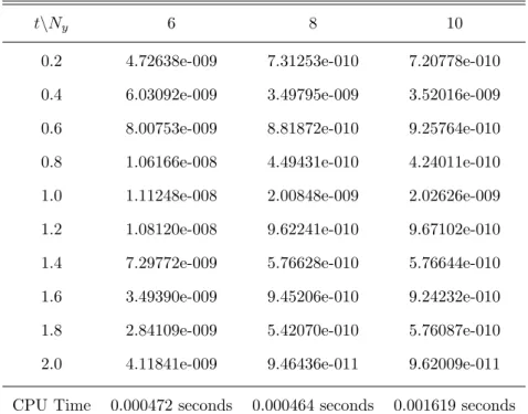
The BSQLM is also used to solve the Fisher's equation and the infinity standard errors are shown in Table 5.8. When ISQLM was used, the infinity norm errors show an increase as the collocation points Ny increase giving an infinity norm error of up to 10−6. Comparing the CN-SQLM with the BSQLM, it is clear that BSQLM gives much better results with an infinite norm errors of up to 10−11.
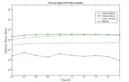
The infinity standard errors for both methods are plotted and shown in Figure 5.2 which are consistent with the results in Tables 5.5 - 5.8.
The Burgers-Fisher Equation
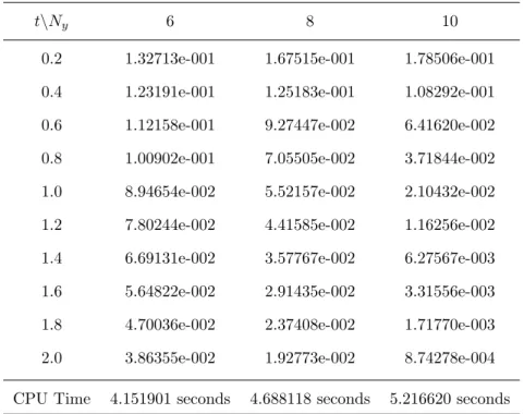
The infinite norm error given in Table 5.12 was obtained using 10 collocation points in both variables and y. Accordingly, Table 5.12 shows the infinite norm errors for the Burgers-Fisher equation using BSQLM. The processor time increases as the number of collocation points increases and as t → 2, the error of the infinite norm decreases.
In the results for SQLM, using an explicit method, implicit method and Crank-Nicolson and the BSQLM, it is observed that the infinity norm errors improve as t → 2. Second, it is noted that as the number of collocation points increases, the infinity norm errors decrease significantly . The infinity norm errors in general for this example are poor and only give up to 10−4 for SQLM and are better for BSQLM as they increase to 10−10.
The infinity norm error graph is shown in Figure 5.3, which also agrees that BSQLM is a better method than SQLM.
Newell-Whitehead-Segel and Zeldovich Equations
From Table 5.13 and Table 5.14 it can be seen that the infinite norm error decreases as the number of collocation points Ny increases and the CPU time increases. It is clear from Table 5.15 that as Ny increases, the infinite norm error decreases and the CPU time increases as the number of collocation points increases. The results of the infinite norm error using the Bivariate Spectral Quasilinearization method for the Newell-Whitehead-Segel equation are given in Table 5.16, which was obtained using an equal number of collocation points intandy variables, equal to 10.
When t = 0.4, ESQLM and ISQLM give the minimum infinity rate error compared to CN-SQLM. In the same figure, from t ≥ 1.4 to t= 2, the infinity rate error of CN-SQLM decreases. The infinity rate error results are shown in the tables and their CPU time for SQLM.
Finally, the Zeldovich equation was solved and the infinite norm errors are shown in Tables for SQLM and Table 5.20 for BSQLM.
Comparative Discussion
These tables were obtained by using an equal number of collocation points in the spatial direction Ny and in the time variable, Nt = 100 for all other examples except Fisher's equation and the Zeldovich equation. It is noted that for Fisher's and Zeldovich equations an increase in the collocation points in the time variable reduces the infinity norm errors, while in the other examples there is no significant change in the results if Nt is increased. It is clear from the comparison of the computational running times (CPU time) that BSQLM takes less computer time than SQLM.
Furthermore, the results indicate that for both methods the computation time also increases as the number of collocation points in the space variable increases. The actual superiority of the BSQLM in terms of arithmetic ability and accuracy compared to the SQLM can be elucidated by the fact that the SQLM scheme used the finite difference time derivative, which has been proven in the literature to be less accurate than the spectral methods. Although different collocation points were used, the BSQLM seemed to give much less infinite error norm, and also required fewer collocation points.
Therefore, the BSQLM is a better method that can be used to obtain numerical solutions of nonlinear partial differential equations than the SQLM.
Overview
Darvishi, "En numerisk løsning af Burgers' ligning ved modificeret Adomian-metode", Applied Mathematics and Computation, vol. Jain, "Numerical Solutions of Nonlinear Fisher's Reaction-Diffusion Equation with Modified Cubic B-Spline Collocation Method", Mathematical Sciences, vol. Abdelkawy, "A Jacobi Collocation Method for Solving Non-linear Burgers- Type Equations" Abstract and Applied Analysis, vol.
Hassanb, "A Chebyshev Spectral Collocation Method For Solving Burgers'-Type Equations", Journal of Computational and Applied Mathematics, vol. Mittal and R.K.Jain, "Numerical Solutions of Fisher's Nonlinear Reaction-Diffusion Equation by Modified B-Spline Cube Summation Method," Mathematical Sciences, vol. Pue-on, "Laplace Adomian Decomposition Method for Solving the Newell-Whitehead-Segel Equation", Applied Mathematical Sciences, vol.
69] Z.K.Jabar, “Numerical solution of the generalized Burger-Huxley finite difference method”, J.Thi-Qar Sci., vol.