Comparison between satellite-based and cosmic ray probe soil moisture estimates : a case study in the Cathedral Peak catchment.

(1)

COMPARISON BETWEEN SATELLITE-BASED AND COSMIC RAY PROBE SOIL MOISTURE ESTIMATES: A CASE STUDY IN THE CATHEDRAL PEAK CATCHMENT

THIGESH VATHER

Submitted in partial fulfilment of the requirements for the degree of MSc in Hydrology

School of Agriculture, Earth and Environmental Sciences University of KwaZulu-Natal

Pietermaritzburg

Supervisor: Ms K T Chetty Co-supervisors: Dr M G Mengistu

Prof C S Everson

November 2015

(2)

ABSTRACT

Soil moisture is an important hydrological parameter, which is essential for a variety of applications, extending to numerous disciplines. Currently, there are three methods of estimating soil moisture. These include: (a) ground-based (in-situ) measurements, which are carried out using field instruments; (b) remote sensing based methods, which use specialized sensors on satellites and aircrafts and (c) land surface models, which use meteorological data as inputs, at a predefined spatial resolution (Albergel et al. (2012); Mecklenburg et al., 2013).

In recent years the cosmic ray probe (CRP), which is an in-situ technique, has been implemented in several countries across the globe. The CRP provides area-averaged soil moisture at an intermediate scale and thus bridges the gap between in-situ point measurements and satellite-based soil moisture estimates (Zreda et al., 2012). The aim of this study was to first evaluate the current techniques for soil moisture estimation, in order to identify the research gaps and limitations. The key objectives of this study were to test the suitability of the CRP to provide spatial estimates of soil moisture and use these estimates to validate satellite-based (remote sensing and modelled) soil moisture estimates in the Cathedral Peak Catchment VI. The CRP was set-up and calibrated in Cathedral Peak Catchment VI. An in-situ soil moisture network was created in Catchment VI, which was used to validate the calibrated CRP soil moisture estimates. Once calibrated, the CRP was found to provide spatial estimates of soil moisture, which correlated well with the in-situ soil moisture network dataset and yielded a R² value of 0.8445. The calibrated CRP was used to validate satellite-based soil moisture products. The remote sensing products used were the Level Three AMSR2 and SMOS products. The AMSR2 and SMOS products generally under-estimated soil moisture throughout, but followed the general trend of the CRP, with AMSR obtaining a R² of 0.505 and SMOS obtaining a R² of 0.4853, when compared against the CRP estimates. The CRP was used to validate modelled soil moisture products, which consisted of the SAHG product and the back-calculation of soil moisture, using equations by Su et al. (2003) and Scott et al. (2003), and products derived from the SEBS Model. The SAHG Model performed well, as it provided estimates that correlated well with the CRP dataset and yielded a R² value of 0.624 compared to the CRP estimates. The SEBS back- calculation technique performed very poorly, as it over-estimated in the wet periods and under-estimated in the dry periods.

(3)

DECLARATION

I, Thigesh Vather, declare that:

(i) the research reported in this dissertation, except where otherwise indicated, is my original work.

(ii) this dissertation has not been submitted for any degree or examination at any other university.

(iii) this dissertation does not contain other persons’ data, pictures, graphs or other information, unless specifically acknowledged as being sourced from other persons.

(iv) this dissertation does not contain other persons’ writing, unless specifically acknowledged as being sourced from other researchers. Where other written sources have been quoted, then:

(a) their words have been re-written, but the general information attributed to them has been referenced;

(b) where their exact words have been used, their writing has been placed inside quotation marks, and referenced.

(v) Where I have reproduced a publication of which I am an author, co-author or editor, I have indicated, in detail, which part of the publication was actually written by myself alone and have fully referenced such publications.

(vi) This dissertation does not contain text, graphics or tables copied and pasted from the Internet, unless specifically acknowledged, and the source being detailed in the Dissertation and in the References sections.

Signed: ………..

Thigesh Vather

Supervisor: ………..

Miss Kershani Tinisha Chetty

Co-supervisor: ………

Dr Michael Mengistu

(4)

PREFACE

The work undertaken and described in this dissertation was carried out in the Centre for Water Resources Research (CWRR), in the School of Agriculture, Earth and Environmental Science. This school is within the University of KwaZulu-Natal, Pietermaritzburg. The following dissertation was supervised by Ms KT Chetty, Dr MG Mengistu and Prof CS Everson.

This dissertation is original, unpublished, independent work by the author Thigesh Vather.

The work of other authors, when used, has been given the appropriate credit.

(5)

ACKNOWLEDGEMENTS

The following Masters Research titled “Comparison Between Satellite-Based and Cosmic Ray Probe Soil Moisture Estimates: A Case Study in the Cathedral Peak Catchment’’ has been funded by the Centre for Water Resources Research (CWRR) and the National Research Foundation (NRF). I am grateful for the aforementioned institutions for the funding they have contributed towards this research. I would also like to acknowledge the following people and institutions for their fundamental role in the completion of this research project:

First and foremost, I would like to thank my parents and sisters for their continuous love and support. I appreciate all that you have done for me, not only during the past two years, but throughout my life Thank you to my extended family and friends for all the love and support you have given me. Thank you to Vadinie Moodley, for all the love and support, as well as keeping me focused throughout my Masters.

 Miss KT Chetty (supervisor). Thank you for your guidance and support throughout the duration of the research project. Your mentorship has been of much value to the completion of the dissertation.

 Dr MG Mengistu (co-supervisor). Thank you for all the support and mentorship. Your contribution towards the completion of this research study has been invaluable. Thank you for all the field trips to Cathedral Peak and assisting me will all the aspects of my project, such as the setting up of the cosmic ray probe, setting up of the soil moisture network, calibrating the cosmic ray probe, teaching me how to set-up and run the SEBS model and for assisting with any problems that arose.

 Prof CS Everson (co-supervisor). Thank you for all the support and mentorship throughout the project. Thank you for making this research project possible by obtaining the cosmic ray probe. Thank you for all the well organized and productive field visits. Thank you for assisting me with the various fieldwork activities that were carried out. Thank you for organizing the various instrumentation and support throughout the project.

(6)

 Mrs S Rees. Thank you for assisting me with the editing of the dissertation. I really appreciate the time and effort that you have put into improving the dissertation.

 Mr S Mfeka and Mr C Pretorius. Thank you for all the assistance in the field and the laboratory. Thank you for always being willing to help and always approachable.

 The winter school. Thank you for assisting me with the first calibration, which was the most labour intensive and time consuming calibration. I appreciate all the work and effort that was made.

 Prof TE Franz. Thank you for assisting me with the third calibration, as well as teaching me the cosmic ray probe calibration procedure.

 Dr S Sinclair. Thank you for the assistance in providing the PyTOPKAPI soil moisture product.

 Mr S Gokool. Thank you for your assistance and advice throughout the duration of the project. Your suggestions towards improving the project were greatly beneficial and appreciated.

 Mr B Scott-Shaw. Thank you for assisting with the fire breaks.

 Mrs S van Rensburg. Thank you for organizing the accommodation and other aspects of the field trip. The work and effort that you have contributed is greatly appreciated.

 Thank you to the Staff and Students of the Hydrology Department for all the help and continuous support.

(7)

LIST OF TABLES

Page

Table 2.1 Advantages of the CRP ... 11

Table 3.1 Evaluation of downscaling techniques ... 22

Table 6.1 Geographical coordinates of sample points ... 41

Table 6.2 Variables required in obtaining the bulk density ... 48

Table 6.3 Information regarding the calibration sampling... 49

Table 6.4 The gravimetric soil moisture, bulk density and Neutron count ... 57

Table 6.5 Date and calculated No value for each calibration ... 58

Table 6.6 The bulk density of Catchment VI, as determined by Everson et al. (1998) ... 79

Table 6.7 Mean bulk density according to depth ... 79

Table 6.8 Characteristics of the various landsat 8 bands (USGS, 2015). ... 81

Table 6.9 Calculated ESUN values ... 84

Table 6.10 Zonal statistics of relative evaporation enclosed by catchment VI ... 92

Table 7.1 T-test of In-situ against CRP estimates ... 98

Table 7.2 T-test of CRP against AMSR2 estimates ... 103

Table 7.3 T-test of CRP against SMOS estimates ... 110

Table 7.4 T-test of CRP against SAHG estimates ... 118

Table 7.5 Relative evaporation and evaporative fraction calculated using the SEBS model for Catchment VI ... 120

Table 7.6 Evaporative fraction estimates from the SEBS Model and eddy covariance technique ... 126

(11)

LIST OF FIGURES

Figure 2.1 CRP system in Cathedral Peak Catchment VI ... 7

Figure 2.2 Difference in neutron concentration according to soil moisture content (Franz et al., 2012b). ... 9

Figure 2.3 Measurement area and depth of CRP (Ochsner et al., 2013) ... 10

Figure 3.1 AMSR2 sensor on-board the GCOM-W1 satellite ... 16

Figure 3.2 SMOS satellite ... 18

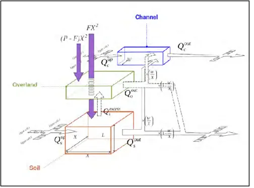
Figure 4.1 A schematic of the water transfer in a typical PyTOPKAPI model cell (Sinclair and Pegram, 2012) ... 26

Figure 4.2 Data-flow diagram showing sources of the dynamic and static data to produce the main information streams (Sinclair and Pegram, 2010). ... 27

Figure 6.1 Location of Cathedral Peak Catchment VI, within the Tugela catchment, within KwaZulu-Natal ... 37

Figure 6.2 Topographic map of Catchment VI ... 38

Figure 6.3 CRP in Cathedral Peak Catchment VI ... 39

Figure 6.4 Diagram of sampling points ... 40

Figure 6.5 Position of calibration sample points within Cathedral Peak Catchment VI ... 41

Figure 6.6 Field samples contained in plastic bags ... 42

Figure 6.7 Weighing the soil samples and placing them in the oven ... 43

Figure 6.8 (a) Setting up the TDR pit, (b) Wireless TDR, (c) Echo probe and (d) Data Hobo Onset logger for the Echo probe ... 44

Figure 6.9 Data retrieved from burned echo probe data loggers ... 46

Figure 6.10Protection of equipment by fire breaks in Catchment VI ... 46

(12)

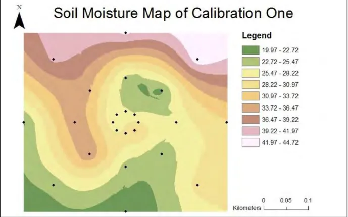
Figure 6.11Soil moisture map of the first calibration (9th of July 2014) ... 50

Figure 6.12Soil moisture map of the second calibration (28^th of August 2014) ... 50

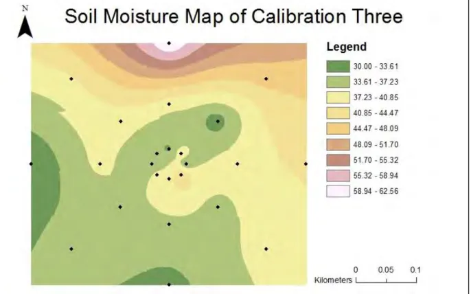
Figure 6.13Soil moisture map of the third calibration (2^nd of December 2014) ... 51

Figure 6.14Soil moisture map of the fourth calibration (22^nd of January 2015) ... 51

Figure 6.15Volumetric water content against depth for each replicate at one sample point ... 52

Figure 6.16Volumetric water content against depth for all 24 sample points ... 53

Figure 6.17Hourly temperature (The same data gaps present in the relative humidity dataset) ... 55

Figure 6.18Complete daily air temperature data for Cathedral Peak Catchment VI ... 56

Figure 6.19CRP soil moisture estimates prior to calibration, with calibration points ... 58

Figure 6.20Hourly soil moisture estimates of the calibrated CRP ... 59

Figure 6.21Neutron count against volumetric water content ... 59

Figure 6.22Daily calibrated CRP soil moisture measurements in Catchment VI ... 60

Figure 6.23Daily TDR pit soil moisture measurements in Catchment VI ... 61

Figure 6.24The CRP effective measurement depth ... 62

Figure 6.25The average TDR pit soil moisture measurements in Catchment VI ... 62

Figure 6.26Daily wireless TDR data in Catchment VI ... 63

Figure 6.27Daily echo probe data in Catchment VI ... 63

Figure 6.28Representative soil moisture measurements ... 64

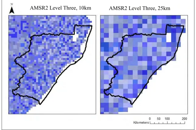
Figure 6.29Comparison of spatial resolution of AMSR2 10 km and 25 km Level Three soil moisture products ... 65

(13)

Figure 6.30The Catchment VI shapefile overlaid over the AMSR2 soil moisture

product to obtain the volumetric water content ... 66

Figure 6.31Navigation through the THREDDS service ... 68

Figure 6.32Layout of the Godiva2 online visualization tool ... 69

Figure 6.33The position of the catchment in relation to a single pixel of the SMOS soil moisture product ... 70

Figure 6.34Godiva2 visualization tool showing the pixel value for the Catchment VI ... 71

Figure 6.35AMSR2 data availability for the observation period ... 72

Figure 6.36SMOS data availability for the observation period ... 72

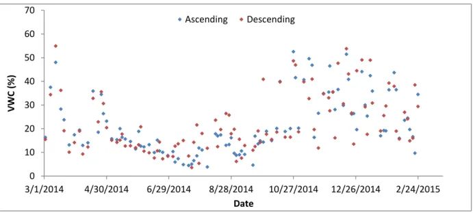
Figure 6.37Time series analysis of days which have both ascending and descending AMSR2 values ... 73

Figure 6.38Time series analysis of days which have both ascending and descending SMOS values... 73

Figure 6.39Navigation through the SAHG website to download SSI data ... 75

Figure 6.40One day of SSI data (eight images on a three hour interval) ... 76

Figure 6.41Daily SAHG soil moisture product ... 77

Figure 6.42Overlay of the Cathedral Peak Catchment VI onto the SAHG soil moisture product ... 77

Figure 6.43Landsat 8 satellite... 80

Figure 6.44Landsat 8 image footprint ... 81

Figure 6.45Landsat images with different cloud-cover conditions ... 82

Figure 6.46Albedo map generated in ILWIS ... 85

Figure 6.47NDVI map generated in ILWIS ... 86

(14)

Figure 6.48Surface emissivity map generated in ILWIS ... 87

Figure 6.49Land surface temperature map generated in ILWIS ... 88

Figure 6.50DEM map used in ILWIS as an input in SEBS ... 88

Figure 6.51The SEBS model in ILWIS ... 89

Figure 6.52Evaporative fraction map generated as an output of the SEBS model in ILWIS... 90

Figure 6.53Relative evaporation map generated as an output of the SEBS model in ILWIS... 90

Figure 6.54Catchment VI shapefile overlaid onto relative evaporation map ... 91

Figure 6.55The relative evaporation map of Catchment VI ... 91

Figure 6.56Processes used to obtain relative evaporation from Landsat 8 data ... 93

Figure 7.1 Daily rainfall measured at Catchment VI ... 95

Figure 7.2 Daily in-situ and CRP soil moisture estimates for Catchment VI ... 96

Figure 7.3 Scatterplot of In-situ soil moisture estimates against CRP estimates ... 97

Figure 7.4 Residual graph of In-situ against CRP soil moisture estimates ... 98

Figure 7.5 Time series analysis of CRP and AMSR2 soil moisture estimates... 100

Figure 7.6 Comparison between summer and winter images of AMSR2 soil moisture estimates ... 101

Figure 7.7 Scatterplot of CRP against AMSR2 soil moisture estimates ... 102

Figure 7.8 Residual graph of CRP against AMSR2 soil moisture estimates ... 103

Figure 7.9 A day with a descending and a day with an ascending value for the AMSR2 soil moisture product ... 104

(15)

Figure 7.10A day with both an ascending and descending value, and a day with no

value for the AMSR2 soil moisture product ... 105

Figure 7.11Time series analysis of CRP and SMOS soil moisture estimates for Catchment VI ... 106

Figure 7.12Ascending SMOS image in summer (17 December 2014) ... 107

Figure 7.13Descending SMOS image in summer (17 December 2014) ... 107

Figure 7.14Ascending SMOS image in winter (15 August 2014) ... 108

Figure 7.15Descending SMOS image in winter (15 August 2014) ... 108

Figure 7.16Scatterplot of CRP against SMOS soil moisture estimates... 109

Figure 7.17Residual graph of CRP against SMOS soil moisture estimates ... 109

Figure 7.18SMOS missing data within band ... 110

Figure 7.19AMSR2, SMOS and CRP soil moisture estimates against time ... 111

Figure 7.20Three-day averaged soil moisture estimates ... 112

Figure 7.21Time series analysis of SAHG and CRP soil moisture estimation ... 114

Figure 7.22SAHG daily soil moisture (summer) ... 115

Figure 7.23SAHG daily soil moisture (winter) ... 116

Figure 7.24Scatter graph of CRP against SAHG soil moisture estimates ... 117

Figure 7.25A residual graph of CRP against SAHG was plotted against time ... 118

Figure 7.26A range of different relative evaporation images for Catchment VI ... 121

Figure 7.27A range of different evaporative fraction images ... 122

Figure 7.28Time series of CRP estimates and soil moisture back-calculated from the SEBS model ... 123

(16)

Figure 7.29Scatter graphs of CRP against the SEBS Model estimates a) CRP against Su et al. (2003) and b) CRP against Scott et al. (2003). ... 124

Figure 7.30Residual graph of CRP against Su et al. (2003) and Scott et al. (2003). ... 125 Figure 7.31Time series of the CRP soil moisture estimates and soil moisture from the

Scott et al. (2003) method using the evaporative fraction from SEBS and the eddy covariance method. ... 127 Figure 7.32Number of observation days per month that data was available for each

product ... 129

(17)

LIST OF SYMBOLS

q_p₌ Pore water content (g/g) rbd = Dry soil bulk density (g/cm³) qLW = Lattice water content (g/g)

q_SOC_eq = Soil organic carbon water content (g/g) rv = Absolute humidity of air (g/m³)

AL = Band specific additive rescaling factor Ap = Band specific additive rescaling factor BWE = Biomass water equivalent (mm)

CI = High-energy intensity correction factor CP = Pressure correction factor

CS = Geomagnetic latitude scaling factor CWV = Water vapour correction factor d = Earth sun distance

E = Evaporation (mm)

eo = Actual vapor pressure at surface (Pa) eso = Saturated vapor pressure at surface (Pa) Go = Soil heat flux energy (Wm^-2)

H = Sensible heat flux energy (Wm^-2) Hdry = Sensible heat flux at the dry limit (Wm-²)

(18)

Hwet = Sensible heat flux at the wet limit (Wm^-2) Io = Irrigation (mm)

Lλ = TOA spectral radiance (Watts/ (m2*srad*µm)) ML = Band specific multiplicative rescaling factor Mp = Band specific multiplicative reflectance factor Ms = Mass of soil (g)

Mt = Mass of total (g)

Mvap = Molar mass of water vapor (= 18.01528 g/mol = 0.01801528 kg/mol) N = Corrected neutron counts (counts/hour)

N’ = Raw moderated neutron counts (counts/hour) Ɵ = Volumetric soil moisture (m3.m^-3)

Ɵr = Residual volumetric soil moisture (m3.m^-3) Ɵsat = Saturated volumetric soil moisture (m3.m^-3) P = Pressure (mb)

Po = Precipitation (mm) Ps = Particle density (g/cm3) pλ = TOA planetary reflectance

pλ’ = TOA planetary reflectance (without solar angle correction) Qcal = Quantized and calibrated standard product pixel value (DN) R = Universal gas constant (= 8.31432 J/mol/K)

RH = Relative humidity (%)

(19)

Rn = Net radiation (Wm^-2)

Rvap = Gas constant for water vapor (J/K/kg) T = Air temperature (^oC)

t = Time (s)

TC = Soil total carbon (g/g)

Ts = Land surface temperature (K) Z = Vertical distance (m)

α = Land surface albedo (dimensionless) εo = Surface emissivity (dimensionless) ΘSE = Local sun elevation (degrees) λE = Latent heat flux energy (Wm^-2) λEdry = The latent heat at the dry limit (Wm^-2) λEwet = The latent heat at the wet limit (Wm^-2) Λr = Relative evaporation (dimensionless)

(20)

LIST OF ABBREVIATIONS

AMSR2 : Advanced Microwave Scanning Radiometer

CRP : Cosmic Ray Probe

ESA : European Space Agency

ILWIS : Integrated Land and Water Information System

LST : Land Surface Temperature

NDVI : Normalized Difference Vegetation Index

PyTOPKAPI : Python Topographic Kinematic Approximation and Integration SAHG : Satellite Applications and Hydrology Group

SEBAL : Surface Energy Balance Algorithm for Land SEBS : Surface Energy Balance System

SMOS : Soil Moisture and Ocean Salinity

TDR : Time Domain Reflectometry

TOPKAPI : Topographic Kinematic Approximation and Integration

VWC : Volumetric Water Content

(21)

1. INTRODUCTION

There has been an incessant need to monitor and measure the various parameters in land surface hydrology, in order to deepen the understanding of hydrological processes, their importance in the hydrological cycle and their interactions between each other (Jackson et al., 2010; Fang and Lakshmi, 2014). Soil moisture is an important parameter in the hydrological cycle and greatly impacts a variety of applications, including agricultural management, climate and weather applications, flood and drought prediction and groundwater recharge.

Although soil moisture does not directly contribute to the land surface energy balance, the properties associated with soil moisture have a strong influence on net radiation, and the partitioning between latent and sensible heat fluxes (Wang and Li, 2011). Soil moisture is a significant variable in the earth’s water cycle, even though it holds a small percentage of the total global water budget (Guillem, 2010). Weather and climate applications rely greatly on soil moisture, consequently the predication accuracy of global weather forecast models and climate applications may increase, with improved estimates of soil moisture data (Guillem, 2010). Soil moisture is a key component in crop growth and is the prime regulator of a catchment’s response to rainfall, as it partitions rainfall into infiltration and surface runoff (Vischel et al., 2008; Zhao and Li, 2013). Due to the impacts of global change, numerous cycles, such as the hydrological cycle, have been pushed past their thresholds. Therefore, monitoring the soil moisture status of an area, such as a catchment, can assist in mitigating the negative effects of extreme environmental processes or phenomena, such as droughts and floods (Guillem, 2010).

Soil moisture is a difficult parameter to continuously monitor and measure at a catchment scale due to its heterogeneous characteristics. It varies both spatially and temporally and is thus a dynamic resource, which never remains constant. Currently, there are three methods of estimating soil moisture. These include: (a) ground-based (in-situ) measurements, which are carried out using field instruments; (b) remote sensing based methods, which use specialised sensors on satellites and aircrafts and (c) land surface models, which use meteorological data as inputs, at a predefined spatial resolution (Albergel et al., 2012; Mecklenburg et al., 2013).

Inherently each of these methods possess their respective advantages and limitations, constraining their effectiveness for hydrological applications (Ni-Meister, 2005).

(22)

In-situ measurements of soil moisture are the conventional methods used by several disciplines. The point measurements obtained cannot adequately represent the spatial characteristics of soil moisture. However, these point measurements play a key role in a variety of large-scale applications and are invaluable as both calibration and validation data (Gruber et al., 2013). In the past few years, the Cosmic Ray Probe (CRP) method, which is an in-situ instrument, has been developed and implemented in numerous countries across the globe (Kohli et al., 2015). The CRP technique obtains the area-averaged soil moisture, at an intermediate scale, by observing and measuring the cosmic ray neutrons above the soil surface (Zreda et al., 2012; Franz et al., 2013).

Remote sensing can be described as the technique of obtaining information about an object or phenomena, with the use of special instrumentation from a distance, without making physical contact (Engman, 1991; Wagner, 2008; Mekonnen, 2009; Lakshmi, 2013). Remote sensing is extensively used today by several disciplines to observe and measure various environmental parameters. Hydrology is one such discipline, which uses remote sensing to measure parameters, such as rainfall, evaporation and surface temperature (Fang and Lakshmi, 2014).

There are several remote sensing soil moisture estimating techniques, which use gamma, near infrared, microwave and thermal radiation. The passive microwave radiation technique is the most commonly used technique, as it has several advantages over other techniques. The passive microwave technique observes and measures the difference in dielectric constants of dry soil and water to estimate soil moisture (Jackson et al., 2010; Lakshmi, 2013). Currently, the microwave remote sensing soil moisture products are available on a global scale;

however, these products are limited by their coarse spatial resolution, which is inadequate for hydrological applications (Shin and Mohanty, 2013; Song et al., 2013). Therefore, downscaling techniques have been researched and developed, to obtain soil moisture at a finer spatial resolution. (Lakshmi, 2013).

Models have been used to obtain estimates of soil moisture at an intermediate scale. A model implies a simplification of reality and aims to promote understanding, whilst simplifying and mimicking the real system. Soil moisture is an important variable in both the land surface energy and water balance and can be estimated from surface energy balance models, such as the Surface Energy Balance System (SEBS) and land surface water models, such as the Topographic Kinematic Approximation and Integration Model in Python (PyTOPKAPI).

(23)

The objective of this study is to review literature pertaining to the current methods of soil moisture estimation, which include in-situ, remote sensing and modelling. This is required to broaden the understanding of this field of study. This will aid in identifying the commonalities and gaps in the literature, as well as the key methods used and their limitations in the estimation of soil moisture. The key focal aspects of the literature review are to evaluate the CRP for use as a validation method. In addition, the current methods of remote sensing soil moisture products will be reviewed and the modeled soil moisture estimates will be analysed. The aim of the study is to test and evaluate the suitability of the CRP to provide spatial estimates of soil moisture in Cathedral Peak Catchment VI and use these estimates to validate satellite-based soil moisture estimates. Satellite-based soil moisture products comprise of remote sensing soil moisture products and models, which use remote sensing data as inputs.

The Research questions include:

i. How suitable is the CRP method in providing spatial estimates of soil moisture in Cathedral Peak Catchment VI?

ii. How well do remote sensing soil moisture products compare to the CRP estimates?

iii. How well do modelled soil moisture products compare to the CRP estimates?

The dissertation is divided into eight chapters, starting with the introduction in chapter one.

The literature review is not a single chapter but is encompassed in chapters two, three, four and five. Chapter two outlines the in-situ methods of soil moisture measurement, which consists of conventional in-situ methods, as well as the CRP. Chapter three outlines the remote sensing of soil moisture and focuses on the current global soil moisture products.

Chapter four outlines the use of modelling to obtain soil moisture estimates. Chapter five is the literature evaluation, which looks at the general themes in soil moisture measurements and evaluates the gaps in the literature reviewed. Chapter five is an important chapter, as it summarizes the evaluated literature and sets the foundation for the methodology, which is presented in chapter six. The methodology is presented in chapter six, which outlines the study area, as well as details the various procedures and techniques that were used in this research study. Chapter seven contains the results and discussion of the research study. The conclusions, limitations and recommendations of the study are discussed in chapter eight.

(24)

2. IN-SITU METHODS OF SOIL MOISTURE MEASUREMENT

The following section is the first component of the literature review. The remaining components of the literature review will be covered in the third and fourth chapters. A literature evaluation will be presented in chapter five.

In-situ soil moisture techniques are the conventional methods of soil moisture estimation.

There are numerous in-situ techniques, both direct and indirect, which have been used to determine soil moisture. In recent years, the use of the CRP to measure soil moisture has gradually attracted attention and has been implemented in a number of countries across the world (Villarreyes et al., 2013). The ensuing section will provide an analysis of the conventional methods of soil moisture estimation, which will be followed by a detailed review of the CRP.

2.1 Conventional Methods of Soil Moisture Estimation

In-situ soil moisture measurements have played a key role for a variety of large-scale applications and have been invaluable as calibration and validation data for satellite-based products, sensors and models (Gruber et al., 2013). There are several conventional in-situ techniques used to estimate soil moisture, including the gravimetric method, neutron scattering and Time Domain Reflectance (TDR) (Walker et al., 2004). Brief descriptions of the aforementioned techniques are discussed below:

i. The gravimetric method is a direct method of estimating the soil moisture content.

This method consists of collecting soil samples at points at desired depths. The collected soil samples are then weighed, before being oven-dried for 24-72 hours at 105 ^oC, until all the moisture has been driven out of the sample. The dry samples are then re-weighed. The gravimetric soil moisture is then calculated by dividing the mass of water by the mass of dry soil.

This method is commonly used as it has the advantage of being accurate, is independent of soil type and is easily calculated (Hillel, 2008). However, it is a destructive technique that is time and labour-consuming (Zazueta and Xin, 1994).

(25)

Due to its destructive nature, it does not allow for repetitive sampling at the same point. The method also requires a laboratory equipped with an oven and the time of the sample collection to the time that the samples are weighed has to be minimal, to avoid the loss of moisture from the soil (Hillel, 2008).

ii. The neutron scattering method is an indirect in-situ measurement, which has been used since the 1950’s (Jones et al., 2002). The neutron probe uses an active source of fast neutrons, which pass through the soil and collide with the soil media. These fast neutrons thus slow down with each collision and become slow neutrons. The majority of these fast neutrons collide with hydrogen in the form of water in the soil media.

Thus, the more water present in the soil media, the more hydrogen and the more collisions occur. The measured slow neutrons are therefore proportional to the soil water.

iii. According to Zazueta and Xin (1994), this method has the advantage of being accurate (once calibrated) and able to measure soil profiles, with the measurement being directly related to soil moisture. However, the method is limited because of its cost, radiation hazard, the skills required and the difficulty to obtain accurate measurements near the surface, because it is time-consuming and its invasive nature, as access tubes have to be placed vertically into the soil profile.

iv. The TDR method is a common indirect in-situ method. According to Jones et al.

(2002), there are different variations of TDR probes, but in general, the probe consists of two to three steel rods, which can be placed vertically or horizontally into the soil.

The probe or logger sends out high frequency pulses in the Giga Hertz (GHz) range, which have a varying travel time along the wave guides(stainless steel rods), due to the dielectric constant of the medium in which the probe is placed. The dielectric constant is mostly dependent on the water content of the soil. The TDR probe is insensitive to soil composition and texture, due to the large disparity of dielectric constants, but needs calibration with soils with a high electrical conductivity (Jones et al., 2002).

The TDR method is a commonly used and accurate method, due to its minimal calibration requirements, easily obtainable measurements, low cost compared to other

(26)

methods, and its ability to provide non-destructive continuous measurements (Jones et al., 2002; Walker et al., 2004). The TDR method is limited, as a calibration procedure is required, the depth measured is dependent on the length of the steel rod used and errors may occur from soil voids around the probes measurement area (Zazueta and Xin, 1994; Walker et al., 2004) .

The major limitation of all conventional in-situ methods is that they provide point measurements, which do not account for the spatial characteristics of soil moisture (Qin et al., 2013). Therefore, no single point measurement can be entirely representative of larger areas, because of the heterogeneity that exists in soil properties, topography and weather (Gruber et al., 2013). In order to overcome this limitation, dense soil moisture networks can be set up. However, the high costs of operation and maintenance make the setup of the network financially unfeasible (Gruber et al., 2013).

2.2 Cosmic Ray Probe

Understanding the variability of soil moisture, is of great interest for various disciplines (Villarreyes et al., 2013). The CRP is a relatively new technique, which has the capability of providing soil moisture data for large-scale studies. It is the only in-situ technique that can obtain the average soil moisture content over hundreds of meters, something that would require a dense in-situ point measurement network (Zreda et al., 2012; Ochsner et al., 2013).

The CRP method can play a vital role in the calibration and validation of satellite-based soil moisture retrievals and land surface models (Villarreyes et al., 2013).

As shown in Figure 2.1, the CRP system comprises of neutron counters (moderated and bare tubes), a data logger which includes barometric pressure, humidity and temperature sensors, and a telemetry system with antenna to connect to an iridium satellite, and a battery and solar panel for powering the system.

(27)

Figure 2.1 CRP system in Cathedral Peak Catchment VI

Production of cosmic ray neutrons

Cosmic ray neutrons originate in space, where they are produced by the blast waves of exploding stars. Shards of atoms are accelerated and energized, until they eventually reach a high enough speed to break away and escape to the galaxy. Some of these high energy particle flows in space reach the earth’s atmosphere, where they are affected by the earth’s magnetic field (Jiao et al., 2014). The high energy particles are captured into the earth’s atmosphere and collide with atmospheric nuclei to initiate a cascade of secondary cosmic rays (Ochsner et al., 2013). Fast neutrons are created, as these secondary cosmic rays pass through the atmosphere and then through the top few meters of the biosphere, hydrosphere and lithosphere, (Desilets et al., 2010).

These fast neutrons undergo elastic collisions with nuclei present in the soil, thereby losing energy (Desilets et al., 2010). Some of the fast neutrons are adsorbed by the soil during the collision, whilst others will be scattered above the surface of the soil (Jiao et al., 2014). The cosmic ray neutrons lose energy with each collision, therefore high energy neutrons become fast neutrons (in the atmosphere), which further lose energy and become thermal neutrons (in

Satellite link

Neutron tubes

Data logger

Batteries

Pressure, temperature and

humidity sensors Solar panel

(28)

the soil). Due to fast neutrons being strongly moderated by hydrogen present in the environment, their measured intensities relate to changes in soil moisture, as well as other hydrogen sources at the earth’s surface (Zreda et al., 2008; Zreda et al., 2012; Franz et al., 2013).

Moderation of neutrons

According to Ochsner et al. (2013) and Jiao et al. (2014) the moderation process of cosmic ray neutrons depends on three factors:

i. The scattering probability or the elemental scattering cross-section;

ii. The logarithmic decrement of energy per collision; and

iii. The number of atoms of an element per unit mass of material, which is proportional to the concentration of the element and to the inverse of its mass number.

The combination of the abovementioned factors, defines the neutron stopping power of a material (Ochsner et al., 2013). Hydrogen, which is found mainly as water in the soil, plays the most significant role in moderating cosmic ray neutrons in the soil. Hydrogen has an extraordinary high stopping power, as the hydrogen atom has a high probability of scattering a neutron, due to its fairly large elastic scattering cross-section (Jiao et al., 2014). Hydrogen is the most efficient element, with regards to the decrement of energy per collision and has a low atomic mass and makes up a substantial portion of all the atoms in many soils, due to the presence of water in the soil (Jiao et al., 2014). The presence of water within the soil pores plays an important and central role in moderating the concentration of cosmic ray neutrons above the soil surface (Desilets and Zreda, 2013).

Cosmic ray probe measurements

The fast neutrons that are produced in the air and soil travel in all directions between the air and soil, thus creating an equilibrium concentration of neutrons. This equilibrium concentration is shifted due to changes (addition or subtraction) in the hydrogen content of the media. The soil moisture content is estimated by the concentration of low energy cosmic ray neutrons, which are generated within the soil and moderated predominantly by hydrogen,

(29)

before being diffused back into the atmosphere (Zreda et al., 2008). The soil moisture content can therefore be inferred directly from these neutron fluxes (Desilets et al., 2010).

Dry soils are highly emissive, so that neutrons are more efficiently removed from the soil (Zreda et al., 2008). This results in more neutrons escaping to the surface of a dry soil, which will result in a higher concentration of neutrons above the soil surface, see Figure 2.2 (Franz et al., 2012b).

Figure 2.2 Difference in neutron concentration according to soil moisture content (Franz et al., 2012b).

The CRP system consists of two sensors. The moderated sensor (encased in perspex) measures the fast neutrons, which are attributed to the soil moisture, whilst the bare tube measures the slow neutrons, which are attributed to the water above the soil surface (biomass and snow). The fast neutron intensity above the soil surface is inversely proportional to the amount of soil moisture in the soil surface (Kohli et al., 2015).

Measurement footprint and depth of the cosmic ray probe

The CRP senses all hydrogen present within the distance that fast neutrons can travel in air, water, soil and other materials near the earth’s surface. Thus, the measurement distance varies according to the density and chemical composition of the material (Ochsner et al., 2013). The footprint (measurement area) of the CRP, is defined as the area around the probe from which 86% of the counted neutrons arise (Jiao et al., 2014). The footprint is primarily associated

Dry Soil Wet Soil

(30)

with the chemical and physical properties of the air and is inversely proportional to the air density (Jiao et al., 2014).

The radial footprint of the CRP is reliant on the neutron’s ability to travel hundreds of meters from their source, due to the neutrons scattering in the air (Kohli et al., 2015). Hence the scattering properties of air significantly affect the diameter of the footprint (Jiao et al., 2014).

When the CRP is placed in a static position a few meters above the ground, it has a radial footprint of 670 meters in diameter at sea level (Zreda et al., 2008). The radial footprint size is inversely proportional to the air density. At high altitudes, the air pressure is lower, which results in a larger footprint. The measurement diameter slightly decreases with increasing soil moisture and with increasing atmospheric water content (Jiao et al., 2014).

The effective depth is the thickness at which 86% of counted neutrons arise, which depends strongly on the soil moisture content (Ochsner et al., 2013). The measurement depth is inversely proportional to the soil moisture content. A measurement depth of 0.72 m is obtained in dry soil and a depth of 0.12 m is obtained in wet soil, so that the effective measurement depth decreases with increasing hydrogen. (Zreda et al., 2008). The decrease in measurement depth according to an increase in soil moisture is nonlinear and the measurement depth is independent of the air density.

Due to the fact that neutrons react with any source of hydrogen near the earth’s surface, the measured neutron intensity represents the total reservoir of neutrons present within the probe’s sensing distance (Ochsner et al., 2013). This includes snow, lattice water, water in soil organic matter, water in vegetation and atmospheric water vapour (Ochsner et al., 2013).

The measurement footprint and depth is shown in Figure 2.3.

(31)

The CRP can be used either in a fixed position or in a moving vehicle. The fixed position is used to obtain continuous measurements of an area, whilst the roving method can be used for mapping large areas (Dutta and D'este, 2013). The technique functions, as the neutron fluxes are a great proxy for land surface water (Desilets et al., 2010). Along with the neutron count rate, the CRP also measures the internal temperature, relative humidity within the logger enclosure and external barometric pressure (Franz et al., 2013).

Advantages of the cosmic ray probe method

The CRP method has several advantages (Zreda et al., 2008; Desilets et al., 2010; Franz et al., 2012b; Franz et al., 2012a; Zreda et al., 2012; Desilets and Zreda, 2013; Franz et al., 2013; Jiao et al., 2014), including:

Table 2.1 Advantages of the CRP

Advantages The method is passive and non-contact (non-invasive) The system is easily automated

The CRP is portable

It has minimal power requirements

Applications not limited to soil moisture (can be used to estimate above-ground biomass and snow depth)

The measurement footprint is at an intermediate scale The measurement depth ranges from 0.12 m to 0.72 m

The method allows for continuous measurements to be obtained The instrument is easily installed above-ground

The CRP provides excellent data sets

The CRP requires low data processing and transmission The method is less affected by the presence of vegetation

The method is insensitive to soil texture, bulk density or surface roughness

(32)

The CRP is a fairly recent instrument used to obtain soil moisture estimates and seems to have no major limitation associated with it. However, the measurement depth and the calibration procedure could be potential limitations of the technique. The measurement depth is not set by the user, but is dependent on the soil moisture status of the measurement area.

The measurement depth of the CRP is generally between 0.12 and 0.72 meters, therefore the CRP technique is limited to measuring soil moisture between this depth range. The calibration procedure is time and labour consuming and it needs to be done correctly in order to provide reliable soil moisture estimates.

The CRP calibration procedure is performed by obtaining corresponding measurements of area-averaged soil moisture and neutron intensity. The area-averaged soil moisture is obtained from many ground-based point measurements, by collecting several soil samples within the CRP measurement area and determining the average gravimetric soil moisture per calibration. The measured neutron intensities need to be adjusted and corrected for variations in location, incoming high-energy particles, atmospheric pressure, absolute humidity and changes in biomass (Franz et al., 2015).

It is recommended that a calibration procedure is carried out for both the dry season and the wet season (Dutta and D'este, 2013). Representative soil samples of the measurement area are required to be analysed, to correct the calibration function for lattice water and water in organic matter (Ochsner et al., 2013).

The potential applications of the CRP make it appealing to scientists in various fields, such as agricultural and ecological monitoring, streamflow forecasting, climate science, drought and flood forecasting, as well as slope stability (Desilets et al., 2010). It should also be noted that the discipline of remote sensing can benefit greatly from this innovative technology, by using CRP measurements for both the calibration and validation of sensors and data products, as it overcomes the spatial limitations of conventional in-situ soil moisture estimates (Desilets et al., 2010). The use of the CRP across different continents results in measurement technique consistency, which would reduce the uncertainties related to in-situ measurements that use a variety of probe types/methods (Kim et al., 2015).

There have been a limited number of studies using the CRP, as the technique is fairly new. A

(33)

i. Zreda et al. (2008) conducted a study in Arizona, USA, on the use of cosmic ray neutrons to estimate soil moisture at an intermediate spatial scale. The study concluded that the CRP permits high resolution long-term monitoring and the large radial measurement footprint makes the CRP method suitable for climate and weather applications, as well as for satellite sensor calibration.

ii. Desilets et al. (2010) looked at implementing the CRP in two ways. The CRP was used to provide stationary measurements in south-eastern Arizona and was used to provide roving measurements in Hawaii. The study concluded that both methods can be implemented with confidence.

iii. Desilets and Zreda (2013) investigated the lateral footprint of the CRP, using a combination of neutron transport simulations and the diffusion theory. The study concluded that the measurement footprint is linearly proportional to the sensor height above the ground and inversely proportional to the air density.

iv. Hawdon et al. (2014) conducted a study, which looked at the set-up and field calibration of the CRP at nine locations across Australia. The nine locations had contrasting soil types, land covers and climates. The results of the study indicated that the generalized calibration function is suitable for relating neutron counts to soil moisture and that it holds for all soil types, except for very sandy soils with lower water contents.

(34)

3. REMOTE SENSING OF SOIL MOISTURE

Remote sensing is currently used to measure various parameters of the hydrological cycle, such as rainfall, evaporation and soil moisture. Remote sensing is seen as a promising technique for soil moisture estimation, as it aims to address the spatial and temporal variability of soil moisture (Zhao and Li, 2013). It has the advantages of being able to measure large scale soil moisture, the data obtained has periodic data updates, its ability to monitor soil moisture in remote areas, its usability and its cost (Sabins, 2007; Mekonnen, 2009; Lakshmi, 2013). The major limitation to the implementation of remote sensing in critical hydrological application is its coarse resolution. The following section gives an overview of the common remote sensing of soil moisture products. This is followed by an analysis and evaluation of the current downscaling techniques that have been developed to obtain soil moisture at a finer spatial resolution.

3.1 Overview of Remote Sensing of Soil Moisture

There are several remote sensing techniques that have been developed and applied, which include gamma radiation, thermal infrared, near infrared and microwave radiation techniques (Albergel et al., 2012). Each technique measures a different land surface quantity, uses a different range of the electromagnetic spectrum and has its own unique advantages and limitations (Mekonnen, 2009). From past research studies, it is evident that the microwave radiation technique, which consists of both active and passive methods, can be considered as the most promising technique for the remote sensing of soil moisture. This is due to its advantages over the other techniques, such as its all-weather capability, large spatial coverage, temporal resolution, measurement depth and vegetative penetration (Wagner, 2008;

Wang and Qu, 2009; Guillem, 2010).

Microwave radiation remote sensing observes the large contrast in the dielectric properties of soil particles and water, as well as the dielectric constant increases, as the soil moisture increases (Mekonnen, 2009; Wang and Qu, 2009). Remote sensing does not measure the soil moisture content directly, therefore mathematical models that describe the association between the measured signal and the subsequent soil moisture need to be derived (Wang and Qu, 2009). Over the past few decades, active and passive microwave remote sensing has

(35)

al., 2013). The L-band range (1 to 10 GHz) is preferably used, as higher frequencies are more affected by perturbation factors, such as vegetation cover and atmospheric effects (Albergel et al., 2012). There have been many research studies on microwave remote sensing products over the past few decades. These products include Soil Moisture and Ocean Salinity (SMOS), the Advanced Microwave Scanning Radiometer (AMSR2), European Remote Sensing Satellite (ERS-1/2) and Advanced Scatterometer (ASCAT) (Dorigo et al., 2011).

The remote sensing of soil moisture has advanced and the product user’s trust in the remote sensing data has increased, as there has been continuous improvements to sensors and the algorithms used to estimate soil moisture (Brocca et al., 2013). The launch of the SMOS satellite, which was the first satellite radiometer dedicated to measure soil moisture over land, emphasized the increased need for the measurement of soil moisture. This is further highlighted by the anticipated launch of the Soil Moisture Active Passive (SMAP) satellite in 2014 (Jackson et al., 2010; Lakshmi, 2013; Song et al., 2013; Fang and Lakshmi, 2014).

Currently, there are several remote sensing soil moisture products. The two most frequently utilized products that appear in recent research literature, are the AMSR/AMSR-E (predecessors of the AMSR2) and SMOS soil moisture products (Brocca et al., 2013). These two products will be detailed in the subsequent sections.

3.2 AMSR2

The global change observation mission (GCOM) is a project for the global long-term monitoring of the earth’s environment. The GCOM consists of two satellites, namely, the GCOM-W and GCOM-C. The GCOM-W1 satellite was launched on the 18^th of May 2012 and is equipped with the AMSR2 sensor (Kim et al., 2015). The AMSR2 sensor on the GCOM-W1 satellite, as seen in Figure 3.1, is the successor to the AMSR sensor on-board the ADEOS-II satellite, which has been operational from December 2002 to October 2003 and the AMSR-E sensor, on-board the AQUA satellite, which has been operational from May 2002 to October 2011 (JAXA, 2013a). The basic performance of AMSR2 will be similar to that of AMSR-E, based on the minimum requirement of data continuity (Imaoka et al., 2010).

(36)

Figure 3.1 AMSR2 sensor on-board the GCOM-W1 satellite

The AMSR2 sensor is a passive microwave scanning radiometer that makes observations at multiple polarizations (both horizontal and vertical) and seven frequency bands, ranging from 6.9 GHz to 89 GHz (Kim et al., 2015). It obtains multi-band observations from the C, X and K bands (Lu et al., 2014). The waves observed are weak and are radiated from the atmosphere and the earth’s surface. It orbits 700 km above the earth’s surface and has a swath of 1450 km. Its antenna rotates once every one and a half seconds, which creates a conical scan pattern, with a scanning interval of 10 km. The scanning method is capable of making one day (ascending) and one night (descending) observation, covering more than 99% of the earth’s surface in two days (Lu et al., 2014).

The AMSR2 sensor estimates several of the parameters, which are predominantly linked to the energy and water cycles, such as precipitation, water vapour, sea-surface temperature, soil moisture and snow depth. The AMSR2 sensor is more advanced than its predecessors (AMSR and AMSR-E). It has a larger main reflector with a 2.0 m antenna diameter, which results in a finer spatial resolution, the addition of a new 7.3 GHz channel to eliminate electro-magnetic wave interference, an upgraded calibration system and it has intensive sunlight shielding, to avoid calibration uncertainties (Imaoka et al., 2010; JAXA, 2013a; Kim et al., 2015)

(37)

According to JAXA (2013b), the AMSR2 Level Two soil moisture product uses auxiliary data in the form of global vegetation coverage ratios. It also uses AMSR2 Level One products, which include 10.6 GHz brightness temperatures (horizontal and vertical polarisations), 36.5 GHz brightness temperatures (horizontal polarization), latitude and longitude and observation date.

The AMSR2 Level Two algorithm uses a simple radiative transfer model. The satellite observed brightness temperature (TB) at the 10.7 GHZ and 36.5 GHz channels, measures the natural microwave emissions from the land surface (Kim et al., 2015). The algorithm assumes that the soil temperature is equal to the vegetation canopy temperature and a constant value of 293 K is used throughout the year (Kim et al., 2015). The AMSR2 soil moisture algorithm assesses the vegetation effects on microwave emissions paths. This is important, as vegetation holds a large amount of moisture and thus needs to be evaluated in order to estimate soil moisture from satellite data. The soil moisture algorithm uses the polarization index and the index of soil wetness, obtained from TB, to simultaneously estimate soil moisture and vegetation moisture. With regards to vegetation, the algorithm uses a look-up table method, where a linear relationship between vegetation water content and optical depth is applied (Kim et al., 2015). A dielectric mixing model is used in the algorithm to convert the dielectric constant into soil moisture content (Kim et al., 2015).

3.3 SMOS

The SMOS satellite system, which is illustrated in Figure 3.2, was launched in November 2009 and consists of a space-borne passive microwave L-band (1.4 GHz) interferometric radiometer (Albergel et al., 2012). The overall aim of SMOS is to provide global surface soil moisture maps with an accuracy of 4% at a 35 – 50 km spatial resolution (Parrens et al., 2012). The SMOS satellite has the ability to obtain measurements at multiple angles, which allows for the retrieval of additional parameters (Kerr et al., 2012). The SMOS system is a Y- shaped instrument, which consists of 69 antennae. The antennae are equally spaced along three arms and view the surface of the earth either through full, or two polarized radiances, in order to provide a full image (Gruhier et al., 2011).

(38)

Figure 3.2 SMOS satellite

SMOS operates by measuring the phase difference of radiation from various incident angles, so that the earth’s surface is frequently viewed at different angles and polarizations (Fang and Lakshmi, 2014). The SMOS soil moisture product has an average spatial resolution of 40 km;

however, this varies from 30-50 km due to, the target area being viewed from multiple angles (Kerr et al., 2010). SMOS has a sun-synchronous orbit at an altitude of 757 km, consequently, the entire earth is covered at least twice in three days, with orbit overpasses at 6:00 (ascending) and 18:00 (descending) local standard time (Leroux et al., 2013; Qin et al., 2013).

L-band radiometry has a high potential for the estimation of surface parameters and has been recognised as the most promising technique to monitor soil moisture over land surfaces and at a global scale (Kerr et al., 2012; Parrens et al., 2012). The L-band is the optimum wavelength range to observe soil moisture, as higher frequencies are more affected by perturbing factors, including atmospheric effects and vegetative cover (Parrens et al., 2012; Mecklenburg et al., 2013). The microwave signal at L-band frequency is primarily driven by surface soil moisture (top 5 cm), effective surface temperature and vegetative opacity, with smaller effects from the atmosphere and surface characteristics, such as bulk density, soil texture and surface roughness (Kerr et al., 2012; Leroux et al., 2013). The soil moisture retrieval algorithm needs to account for all these effects (Kerr et al., 2012).

(39)

The SMOS Level Two retrieval algorithm is physically-based and complex. It uses the polarizations and multi-angular information derived by the SMOS satellite and involves the use of decision trees and direct model inversions (Parrens et al., 2012). The retrieval algorithm was designed to be easily improved and uses SMOS Level 1C data as input and uses two types of auxiliary data, namely, static data (soil texture) and dynamic data (temperature) (Kerr et al., 2012). SMOS provides multi-angular microwave polarimetric brightness temperature (TB), from which a surface soil moisture product is derived (Parrens et al., 2012).

The L-band microwave emission of the biosphere model, which simulates the microwave emission at L-Band range from the soil-vegetation layer is a key component of the retrieval algorithm (Parrens et al., 2012). This is important, as the major difficulty in the estimation of soil moisture, using microwave radiometry is due to the presence of dense overlying vegetation, which attenuates the soil emission and adds its own emission (Parrens et al., 2012).

The retrieval algorithm is based on an iterative approach. The aim of the algorithm is to reduce a cost function, the focal constituent of which is the sum of the squared weighted difference between measured TB and Modelled TB for a collection of incidence angles (Kerr et al., 2012). In order to reduce this cost function, the most suitable set of parameters needs to be determined and used to drive the TB model.

Current remote sensing soil moisture products have a spatial pixel grid between 10 to 50 km.

The major issues in the calibration and validation procedure, when using in-situ point measurements, are the vertical and horizontal scaling issues. The vertical scaling issues occur when remote sensing soil moisture (top 0.05 m) is calibrated and validated against in-situ soil moisture measurements (0.00 to 2.00 m) (Jackson et al., 2010). Therefore, the measurements are at different depths, which is a problem, as soil moisture varies with depth. The horizontal scaling issues occur when a point measurement is used to validate a remote sensing area- averaged value. The assumption that the point is representative of a large area can be conceded to be incorrect, due to the spatial variability of soil moisture (Gruber et al., 2013).

Therefore, there needs to be a shift to area-averaged in-situ methods, to validate and calibrate remote sensing data.

(40)

There have been numerous studies on passive microwave remote sensing for soil moisture estimation. The AMSR-E product is a frequently-used product in past studies. Research studies that have evaluated surface soil moisture derived from AMSR–E, have shown promising results (Koike et al., 2004; Draper et al., 2009; Zhang et al., 2011; Qin et al., 2013). Previous literature has mentioned the launch of the SMOS satellite and how it emphasizes the value of soil moisture estimation in the science field. SMOS data have been used in studies which have shown its potential for accurately obtaining soil moisture measurements (Gruhier et al., 2011; Merlin et al., 2012; Wagner et al., 2012; Mecklenburg et al., 2013; Qin et al., 2013). Over the past few decades, there have been many studies involving both the calibration and validation of remote sensing soil moisture products to in- situ soil moisture measurements (Jackson et al., 2010; Brocca et al., 2011; Fang and Lakshmi, 2014). The following are some of the remote sensing based soil moisture product studies:

i. The AMSR2 soil moisture product has been used in a recent study by Lu et al. (2014), which presented a revised soil moisture retrieval algorithm of AMSR2 and aimed at improving the soil moisture estimates in dry regions. The study concluded that the revised algorithm is effective in overcoming the over-estimation of soil moisture in desert regions.

ii. A recent study by Kim et al. (2015) assessed two versions of the AMSR2 soil moisture product. The AMSR2 product from the Japan Aerospace Exploration Agency (JAXA) and Land Parameter Retrieval Model (LPRM) from the VU University Amsterdam, were used and compared on a global scale against field measurements. The study used CRP measurements from the COSMOS. It concluded that the JAXA AMSR2 product has a relatively better performance under dry conditions; however, the JAXA algorithm generally under-estimates the ground soil moisture. It also indicated that there is a need to improve both the algorithms and that a combined product could provide better estimates of soil moisture.

iii. A study by Leroux et al. (2013), compared the SMOS, AMSR-E and ASCAT soil moisture products over four watersheds in the United States for the year 2010. The study concluded that the SMOS product correlated the closest to ground