Generalized travelling wave solutions for a microscopic chemotaxis model.

(1)

Generalized travelling wave solutions for a microscopic

chemotaxis model

P. M. Tchepmo Djomegni

(2)

Generalized travelling wave solutions for a microscopic chemotaxis model

P. M. Tchepmo Djomegni

This dissertation is submitted in fulfilment of the academic requirements for the degree of Doctor of Philosophy in Applied Mathematics to the School of Mathematics, Statistics and Computer Science, College of Agriculture, Engineering and Science, University of KwaZulu- Natal, Durban.

November 2014

As the candidate’s supervisor, I have approved this dissertation for submission.

Professor K S Govinder ... November 2014

(3)

Abstract

In biology cell migration is one of the most critical processes, for it is decisive in the mechanisms leading to the beginning of life. The collective migration of cells via wave motion plays a key role in understanding many essential steps in developmental processes. It is often modelled as a system of partial differential equations (PDEs). We investigate in a one-dimensional microscopic model, the formation of travelling bands (via wave motion) of bacteria E coli, caused by the chemotactic response of cells to a signal moving with constant speed. We also look at the impact of cell growth and unbiased turning rate on the behaviour of our system. The model derives from the experimental observation reported in Budrene and Berg (1991, 1995).

In the first problem we tackle, we overlook the proliferation of the cells and we search for travelling wave solutions in the case where the cells do not starve. We show that, using a group theoretical approach, a larger class of travelling wave solutions than that obtained from the standard ansatz is possible. By applying realistic initial and boundary conditions, we restrict the general solutions appropriately. This is the first time that explicit travelling wave solutions have been obtained for this system of equations. In particular, we treat the full system, including non-zero diffusivity terms, unlike previous approaches. Importantly, we provide biologically relevant solutions.

The second problem focuses on the metabolism effect in the case of starvation. It was observed experimentally that a low concentration of nutrients may not cause the band to break up, but rather impel the cells to consume the excreted signal. Here cell growth is allowed with constant rate. We use asymptotic methods to prove the existence of travelling wave solutions in both the case of diffusivity and non diffusivity. Significant results have been obtained.

In the last problem we incorporate the proliferation of the cells in the case of non-limiting

(4)

resources. Constant cell growth and a nutrient dependent proliferation rate are considered. We combine a dynamical systems analysis with other analytic methods to investigate the behaviour of the solutions. Travelling wave solutions have been obtained both for high chemotactic sensitivity, and also in the case of no chemotaxis. Explicit, biologically and pertinent solutions have been provided, confirming the validation of the model.

(5)

Preface

I declare that the contents of this dissertation are original except where due reference has been made. It has not been submitted before for any degree to any other institution.

P. M. Tchepmo Djomegni November 2014

(6)

Declaration 1 - Plagiarism

I, Patrick Mimphis Tchepmo Djomegni, declare that

1 The research reported in this thesis, except where otherwise indicated, is my original research.

2 This thesis has not been submitted for any degree or examination at any other university.

3 This thesis does not contain other persons data, pictures, graphs or other information, unless specifically acknowledged as being sourced from other persons.

4 This thesis does not contain other persons writing, unless specifically acknowledged as being sourced from other researchers. Where other written sources have been quoted, then:

a Their words have been re-written but the general information attributed to them has been referenced

b Where their exact words have been used, then their writing has been placed in italics and inside quotation marks, and referenced.

5 This thesis does not contain text, graphics or tables copied and pasted from the Internet, unless specifically acknowledged, and the source being detailed in the thesis and in the References sections.

Signed

(7)

Declaration 2 - Publications

Details of contribution to publications presented in this thesis:

Chapter 2

P. M. T. Djomegni and K. S. Govinder. Generalized travelling wave solutions for hyperbolic chemotaxis PDEs. Math. Biosciences(2014), Submitted.

Chapter 3

P. M. T. Djomegni and K. S. Govinder. Travelling wave solutions in chemotaxis: starvation.

J. Math. Biol. (2014), Submitted.

Chapter 4

P. M. T. Djomegni and K. S. Govinder. Asymptotic analysis of travelling wave solutions in Chemotaxis with nutrients dependent cell growth. J. Theor. Biol. (2014), Submitted.

(8)

Acknowledgments

” Except the Lord build the house, they labour in vain that build it; except the Lord keep the city, the watchman waketh but in vain.” Psalm 127, 1 (KJV)

I thank the Lord Jesus Christ for his grace, guidance and the strengths, that enable me to enjoy and accomplish this work.

My exceedingly gratitude to my supervisor Prof. Kesh Govinder for his excellent coaching. I thank him for introducing me to research, for his patience and advice as well as for the financial support and for the connection with the mathematical community through various conferences, workshops and research summer school.

I also extend my gratitude to the College of Agriculture, Engineering and Science, and to the School of Mathematics, Statistics and Computer Science, at UKZN, for the financial support and for the research facilities provided. These allowed me to peacefully relish my research work.

My thanks to the academic staff of the school for the beautiful moment we had together.

I acknowledge to Canadian government for fully funding my four month visit to the University of Victoria (UVic), Canada. I also thank the training (in advanced numerical analysis) and advice received from Prof. Boualem Khouider and Prof. Florin Diacu, and the conducive research environment provided by the Department of Mathematics at UVic. I appreciate the Mathematical Biosciences Institutes (MBI), USA, for inviting and hosting me for a short term research visit.

My deepest gratitude to my father Mr Djomegni Hubert, my aunt Ms Marthe Dihewou, my cousin Ps Leandre Kwawou and his wife, my brothers and sisters Junior, Bruno, Agnes, Judith and Ariane, for their unfailing love, encouragement and emotional support.

(9)

Sincere thanks to all the members of CMFI church in Durban, my family in Christ, for their love and spiritual support. I particularly thank my Pastors Emile and Isa, my brothers Paul, Dr Collins and Lungani, and my sisters Belise, Londeka, Mbali and Milaine. My special thanks to Siphelele and particularly to Nomzamo for their multiple support.

(10)

Dedication

To my Saviour and my redeemer, the Lord Jesus Christ, for the grace He has given me to accomplish this work

To my dear admirable father Mr Djomegni Hubert for his multiple support

To Mr Robin Moodley and his wife Jennifer for their love, and for the spiritual and emotional support

” Remember the Lord your God. He is the one giving you power to be successful, in order to fulfil the covenant he confirmed to your ancestors with an oath.” Deut 8, 18(NLT)

”If you confess with your mouth the Lord Jesus and believe in your heart that God has raised him from dead, you will be saved.”Rom 10,9 (NKJV)

(11)

Chapter 1 Introduction

1.1 Differential equations and its importance in Biology

The endeavour to understand and predict physical phenomena gave birth to mathematical models, represented in the form of differential or difference equations. Differential equations were formulated for the first time in the mid 17th century by Leibniz and Newton, and were applied to solve problems in geometry and mechanics [49].

In systems biology, modeling differential equations has played a remarkable role. Its has helped to study population dynamics [66], spread of infectious diseases [38, 48], intracellular dynamics [39, 111], drug delivery [53, 90], tumour growth [37, 35] and scar formation [20] amongst others.

Malthus [66] was the first to propose a model for population dynamics. Verhulst [103] later improved the model by considering limiting carrying capacity. Lotka [59, 60] and Volterra [106]

later proposed a model to describe the interaction between two populations. This approach is widely used in epidemiology to study the spread of diseases.

Partial differential equations (PDEs) are often employed to model complex mechanism in Biol- ogy, for they consider multivariational parameters (time, space, intracellular variational). They can be used to study the time-space distribution of cell migration, tumour growth, and pattern formation [63, 64, 29]. Fisher’s equation is one of the most used models to describe the spread of a species from a macroscopic (population-based) level. It was formulated by Fisher [31] as

(14)

follws:

∂u

∂t =ru(1−u) +D∂²u

∂x², (1.1)

whereurepresents the density of the specie,Dis the diffusion coefficient,xis the position, tthe time and r a constant. From a microscopic (individual-based) level, the convection equation is commonly used to describe the transport mechanisms of particles. A typical example is the transport equation describing the velocity-jump process given by

∂p

∂t +∇(vp) =R, (1.2) where p(x, v, t) stands for the particle density at the position x, moving with velocity v at time t, and R describes sources or sinks. In the above equation, it is assumed that there is no interaction between particles.

Given the role that PDEs play in understanding complex phenomena, methods for solving PDEs are vital. With the outstanding work of Lie, group theory via symmetry analysis became the most useful method for finding exact solutions of PDEs. Lie symmetries are used to reduce the numbers of variables and the order of the system, to determine invariant solutions [76, 86]. Although the applications of Lie symmetry analysis involved lengthy expressions, the development of software packages has simplified its implementation.

Depending on the complexity of the equations under study, instead of looking at the exact state of solutions at any position, one may only be interested in the long term behaviour. This approach gave birth to dynamical systems analysis, in which the qualitative behaviour of the solutions are analyzed [96]. We have utilized both approaches in this work.

Despite the methods developed to analyse PDEs, many nonlinear PDEs cannot be solve explicitly. As a result, only particular classes of solutions have been explored. Travelling wave solutions are a special type of solution that have great utility. Their particularity is that they move with constant speed and they preserve their shape profile. Importantly, travelling waves have been observed in chemotaxis [1, 8, 25, 84] – the subject of this work.

(15)

1.2 Partial differential equations in chemotaxis

Chemotaxis is the orientation of species in response to chemoattractants. It plays an important role in the collective migration of cells. It contributes to the recruitment of cells into sites of inflammation or infection, and speeds up the metastasis and atherosclesis process of diseases [18, 21, 34, 70, 71]. Understanding the key factors facilitating chemotaxis enables us to control and predict the trajectory of cells, their self-organization, mutual defense and response to extracellular signaling.

Travelling bands (via wave motion) was observed in chemotaxis systems for the first time in the late 1800s by Engelmann [25, 26], Pfeffer [84] and Beyenrinck [8]. Over the past fifty years, the noteworthy work of Adler [1, 2] has made bacterial chemotaxis one of the better-documented systems in Biology. Adler [1, 2, 3] introduced a population of cells in a capillary tube containing oxygen and nutrients. He observed the formation of two bands of cells. The first band consumed some nutrients and all the oxygen, while the second band consumed the residual nutrients. In both bands, cells move towards higher concentrations. The formation of the bands of cells was also observed without the addition of nutrients [2].

From the macroscopic perspective, Keller and Segel [44, 45, 46] formulated the first model (the K-S model) for chemotaxis depicting the chemotactic behaviour of slime molds. The general form of the K-S model is given by:

∂b

∂t = ∇.(µ(s)∇b)− ∇.(k2(b, s)b∇s) +f(b, s), (1.3)

∂s

∂t = D∇²s−g(b, s), (1.4)

whereb(x, t) represents the bacteria density,s(x, t) is the concentration of the critical substrate, k₂(b, s) is the chemotactic sensitivity function, f(b, s) is the cell proliferation rate function, g(b, s) represents the uptake of substrates by cells or degradation, and µ(s) and D are the diffusion coefficients of bacteria and the substrates, respectively.

Often growth and death are neglected in the mathematical analysis of (1.3)–(1.4) due to their long relative time scale. However, the consideration of this biological process has proved to be important in the behaviour of the system. Lapidus et al [55] observed that zero growth did

(16)

not prevent cells from aggregating, but rather reduced the wave speed. Some classes of growth functions were provided by Kennedy et al[47] leading to travelling wave solutions of constant speed. Biologically, Budrene and Berg [13, 14] observed the formation of new bands of bacteria caused by the proliferation of cells.

The global existence of the solutions of (1.3)–(1.4) was proved under different forms of the chemotactic sensitivity function k₂ [39, 40, 77]. A singularity in the function k₂ was required for the existence of travelling wave solutions in the zero growth scenario [44, 45, 46]. Such a restriction is not realistic in certain contexts, for it can cause the bands of cells to move with unlimited velocity [111]. Nadin et al [73] overcame this unnecessary restriction by adding logistic growth terms.

From the microscopic (cell-based) perspective, Patlak [83] proposed the first model for chemotaxis describing a random walk process of a particle with persistence of direction and external bias. For the case of particles moving independently by alternating run and tumble, Alt [4]

and Othmer et al [80] formulated a model describing the velocity-jump processes, written as follows:

∂

∂tp(x, v, t) +v.∇p(x, v, t) = λ Z

V

T(v, v⁰)p(x, v⁰, t)dv⁰, (1.5) wherep(x, v, t) is the particle density at positionx and timet, moving with velocityv, λis the turning rate, and T(v, v⁰) is the turning kernel representing the probability of a velocity jump (if a jump occurs) fromv⁰ tov.

Intracellular dynamics describing the response of cells to chemical have been represented in general in the form of ODEs as follows [5, 28, 29, 93, 95]:

dy

dt =f(y, S), (1.6)

where y = (y₁, ..., y_M) ∈ R^M are internal state variable, S is the concentration of the stimuli detected, and f is a vector function describing the process. Recently, Xue et al[111] proposed a model that considers the interplay between chemoattractants and nutrients. They also represented in their model signal transduction and metabolism processes. Their model can be used in a variety of biological systems to describe the conflict between two species of a microscopic level (individual behaviour). Under the scenario of zero cell growth and non diffusion

(17)

of substrates, Xue et al [111] obtained travelling wave solutions (without requiring a singular sensitivity). Franz et al [32] considered growth in the situation of starvation. They assumed that cells consumed chemoattractants only (which do not diffuse). They demonstrated the existence of travelling wave solutions, but required a minimal wave speed.

1.3 Model formulation

The model studied in this thesis is inspired by the experimental work of Budrene and Berg [13, 14], Brenner et al [11], and Woodward et al [110]. Moving in a semi solid containing a carbon source of succinate (the nutrient), it was observed that bacteriaE coliconsume succinate and secrete a signal gradient of aspartate, then aggregate in response to the signal, and form different geometric patterns. The size of the aggregate increased as the succinate concentration increased. When the concentration of succinate becomes low, the aggregation does not break up; cells consume aspartate.

Within the cells, mechanisms are developed to enable them to communicate and to respond to stimuli. Such mechanism is called the signal transduction. It is well understood in E coli, whereby cells detect signaling via their transmembrane receptors. In response to the signaling, an enzyme will be excreted within the cell and will facilitate the direction of the movement of the cell [7]. The phosphorylation of CheY (caused by chemorepellents) will result to clockwise rotation of the flagella, and will cause the cell to tumble. The dephosphorylation of CheY (caused by chemoattractants) will drive counter-clockwise rotation of the flagella, and will propel the cell forward [23, 65]. We note that the protein CheY facilitates the issuance of the signal from chemoreceptors to flagella, and that E coli moves by alternating runs and tumbles with constant speed s = 10 −20µm/sec [82]. In the mathematical representation of this intracellular dynamic, two main factors are always considered: fast excitation (rapid decrease in the phosphorylated protein), and slower adaptation (slow return to the prestimulus level).

The model describing this process can be formulated as follows [5, 28, 30, 78, 95]:

dy₁

dt =f₁(y, S) = g(S)−(y₁+y₂)

t_e , dy₂

dt =f₂(y, S) = g(S)−y₂

t_a , (1.7)

where the variable y= (y₁, y₂) describes the signal transduction, S(x, t) is the concentration of

(18)

the signal at position xand timet, the functiong encrypts the first step of signal transduction, and te and ta are the time scale for excitation and adaptation respectively.

In the absence (or at low concentration) of the nutrients, cells consume the excreted signal. A well organized metabolism process takes place within the cells allowing them to survive when resources are limited, and to respond to their surroundings. To model this mechanism, Xue et al [111] assumed that after consuming the nutrient F a variable z₁ is responsible for the secretion of the signal S via the pathway

F →z₁ →S. (1.8)

A low level of nutrients catalytically causes z₁ to give rise to a starving variable z₂ via the pathway

φ−^z→¹ z₂ →φ, (1.9)

where φ represent the reactants/products assumed to be in excess. The model description of this intracellular metabolism is formulated as follows [111]:

dz₁

dt =g₁(z, F) = F(x, t)−z₁

t_f , dz₂

dt =g₂(y, S) = z₁−z₂

t_m , (1.10)

where the variable z = (z₁, z₂) represents the metabolism process, and t_f and t_m are the characteristic time scale for the production of the variable z₁ and z₂, respectively.

From a cell-based point of view, the cell distribution can be described via transport equations for velocity-jump processes as follows:

∂p⁺

∂t +s∂p⁺

∂x +

2

X

i=1

∂

∂y_i(f_i(y, S)p⁺) +

2

X

i=1

∂

∂z_i(g_i(z, F)p⁺) =−λ

−∂S

∂x

p⁺+λ ∂S

∂x

p⁻

+h(F)p⁺, (1.11)

∂p⁻

∂t −s∂p⁻

∂x +

2

X

i=1

∂

∂y_i(f_i(y, S)p⁻) +

2

X

i=1

∂

∂z_i(g_i(z, F)p⁻) = λ

−∂S

∂x

p⁺−λ ∂S

∂x

p⁻

+h(F)p⁻, (1.12)

where p^±(x, y, z, t) represents the cell density at the position x, timet and internal state [y, z], moving with velocity ±s, h is the proliferation rate of the cells, and λ is the turning rate function of the cells. We will choose the turning rate proposed by Xue et al[111] given as

λ ∂S

∂x

=λ₀ 1 +

∂S

∂x

k+|^∂S_∂x|

!

=λ₀

1 +χ∂S

∂x

, (1.13)

(19)

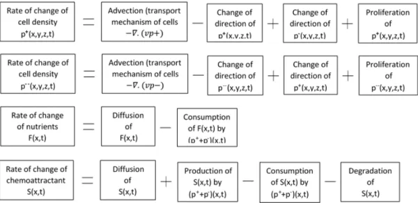
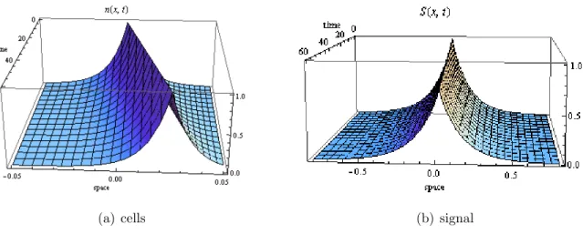
Figure 1.1: Diagram describing the time-space distribution of cells and substrates in chemotaxis with λ₀ being the unbiased turning rate (λ₀ > 0), χ the chemotactic sensitivity and k the sensitivity coefficient.

We can describe using diffusion equations the distribution of substrates as follows [111]:

∂F

∂t =D_F∂²F

∂x² −α₁F Z

Z

Y

w(z₂)(p⁺+p⁻)dydz, (1.14)

∂S

∂t =DS

∂²S

∂x² +α2F Z

Z

Y

w(z2)(p⁺+p⁻)dydz−α1S Z

Z

Y

(1−w(z2))(p⁺+p⁻)dydz−γS,(1.15) where α₁ and α₂ are respective the consumption and production rate of substrates per cell, γ is the degradation rate of the signal, and w is a switch function given by

w(z₂) =







0 for z₂ ≤z_c, 1 for z₂ > z_c,

(1.16)

wherez_cis a critical concentration of succinate that facilitates metabolism. The systems (1.11)–

(1.12) and (1.14)–(1.15) can be interpreted from the diagram in Figure 1.1.

Diffusion of substrates and cell growth and death have often been ignored in chemotaxis models due to the complexity of the analysis. (For instance, the diffusion term involves a higher spatial order in the system, and its non representation reduces the order of the system.) These restric- tions are justified in certain experimental settings (in vivoexperiments, duration of experiment

(20)

taking place before the proliferation process, low diffusion of substrates, etc). However, in many situations they have a significant impact on the behaviour of the system. It was experimentally observed in E colithat the proliferation of cells causes the formation of new bands of cells [14].

Moreover, Elliotet al[24] controlled the migration and the proliferation ofE colicells to invade and interact with tumor cells. Mathematically, it has been proved that allowing diffusion in the model can contribute to the stabilization of the steady state of the system [88].

1.4 Outline

The main objective of this work is to investigate the observed formation of bands of bacteria in our model, via the study of the existence of travelling wave solutions. Unlike previous approaches, we will allow for diffusivity and signal degradation. We will undertake the investigation under the scenarios of growth and of zero growth, and in situations of high sensitivity and non sensitivity to the signal. The effect of microscale parameters such as cell speed, cell growth and unbiased turning rate on the macroscopic behaviour of the system will be examined.

Group theoretical analysis will be used to generate a larger class of travelling wave solutions (via new invariants) than that obtained from the standard ansatz. Only relevant invariants will be considered. The coefficients resulting from the Lie symmetry analysis will play a stabilizing role in the boundedness study of the solutions, confirming our previous findings on the links between group theory and dynamical systems analysis [97]. Generalized travelling wave solutions will be demonstrated, with explicit solutions provided in most of the cases for the first time.

In Chapter 2, we examine the case of non starvation under zero growth. Here, it is assumed that there are enough resources, cells consume nutrients (the succinate) only, and excrete a gradient of signal (the aspartate). We will provide, for the first time, a general form of diffusing solutions.

Realistic initial and boundary conditions will be applied to restrict them appropriately, and to provide biologically relevant travelling wave solutions.

In Chapter 3, we introduce growth and death in the model for non starving cells. Two forms of proliferation rates are considered: constant growth rate and linear growth rate depending on

(21)

the concentration of nutrients. The constant growth is motivated by the observation of Budrene and Berg [14] in which E coli cells grew at a constant rate over the range of 0.5−7mM of succinate concentration. The linear growth rate incorporates both growth and death. We will combine the stability analysis results with asymptotic methods to investigate the behaviour of the system.

In Chapter 4, we look at the scenario of starvation. Starvation in this context depicts the total depletion (or very low concentration) of nutrients. Cells here consume signal only (as observed in [2]). We note that Xue et al [111] in their interpretation of starvation (under zero growth), assumed the possibility of nutrients to be consumed by cells (when the signal concentration becomes the lowest). We here consider the limiting situation of survival (the signal is not produced). We will conduct our analysis under both the cases of zero and constant growth.

Unlike previous approaches, we allow for diffusivity and signal degradation. We will provide explicit solutions in the limiting cases of no chemotaxis and high chemotactic sensitivity.

In Chapter 5, we summarize the results obtained in our analysis. We highlight some limitations to be explored in future work.

(22)

Chapter 2 Travelling wave solutions in chemotaxis under zero growth: no starvation

2.1 Introduction

In biology cell migration is one of the most critical process, for it is decisive in the mechanisms leading to beginning of life. In fact, the signalling of the female reproductive tract is essential in the regulation of sperm motility; most of male sterility results from poor sperm motility [27].

In addition, cell migration is crucial in the growth and maintenance of multicellular organisms via developmental morphogenesis, tissue repair and regeneration as well as tumour metastasis.

It is important to study the collective migration of cells via wave motion, as this plays a key role in understanding many essential steps in developmental processes [108]. For example, in the wound healing process, cells are required to move together in particular directions to specific locations. Additionally, tumor invasion is boosted by proliferation and significant migration of cells into the surrounding tissue [27].

Some bacteria are attracted by nutrients (sugar, amino acids, etc.) and repelled by noxious substances. This phenomenon is called chemotaxis, whereby cells move in response to a chemical gradient (depending on the effect on the cells, the chemical is defined as chemoattractant or chemorepellent) [23]. The chemical activates a receptor at the surface of the cell, which

(23)

results in a physiological response – there is a signal transduction. A well-studied example of this is found in E coli, where bacteria sense the environment and detect chemicals (the signal), mediated by transmembrane chemoreceptors located at the poles. Chemorepellents produce phosphorylation of CheY, which induce clockwise rotation of the flagella, whereas chemoattractants result in CheY dephosphorylation and induce counter-clockwise rotation of the flagella [65]. The chemotaxis protein CheY is involved in the issuance of the signal from the chemoreceptors to the flagella motors [82]. The counter-clockwise rotation pushes the bacterium forward (it is called a “run”), and the clockwise rotation causes the bacterium to tumble, which prevents it from moving toward repellents. In the absence of chemical stimuli, bacteria alternate between run and tumble modes. In Adler’s experiments [1, 2, 3], travelling bands of E coli were observed when a number of cells were introduced at one end of a capillary tube containing oxygen and an energy source. As the amount of oxygen was insufficient to oxidize all the energy sources, two sharp bands of cells, visible to the naked eye, were seen. Cells in the first band consumed the oxygen, excreted and hence caused a gradient in the concentration of oxygen, then moved (at a constant speed) toward higher concentrations. However, in the second band, cells created a gradient in the concentration of the energy source, and moved toward higher concentrations as well. Such phenomena have been formulated by mathematicians in terms of partial differential equations (PDEs) to describe the evolution of cell density and the changes in concentration of chemicals. The established models are classified as linear or nonlinear, discrete or continuous, deterministic or stochastic.

From the macroscopic (population-based) viewpoint, Keller and Segel [44, 45, 46] were the first to propose a continuum model to picture the formation of the chemotactic bands of cellular slime moldsDictyostelium discoideumin response to the chemical. Subsequently, other authors [20, 67, 69] developed discrete models, but the continuum Keller-Segel (K-S) model remained the most popular and the widest used for chemotaxis on population based perspective. The generalized K-S model is written as follows:

∂b

∂t = ∇.(µ(s)∇b)− ∇.(k₂(b, s)b∇s) +g(b, s)−h(b, s), (2.1)

∂s

∂t = D∇²s−f(b, s), (2.2)

where at the position x and time t, b(x, t) stands for the density of bacteria, s(x, t) for the

(24)

concentration of the critical substrate, µ(s) is the diffusion coefficient of bacteria, k₂(b, s) the chemotactic function,g(b, s) andh(b, s) account for the cell growth and death rate functions,D is the diffusion coefficient of the substrate, and f(b, s) is the degradation rate of the substrate.

Often the growth and death terms in (2.1)–(2.2) are overlooked. This is due to the fact that in most cases, these events take place much later than the duration of many in vivo experiments [101]. However, some authors have studied the impact of those terms on the behaviour of the distribution [47, 55, 57, 75]. For instance, Lapidus et al [55] noticed that the absence of bacteria growth did not prevent the aggregation of the cells, but instead decreased the speed of the wave. Kennedy et al [47] identified some classes of functions (standing for the cell growth) which led to travelling wave solutions of constant speed. Lauffenburger et al [57] emphasised the diffusion coefficient, and found that the impact of relative changes in the diffusion coefficient of the population is higher than the relative changes in the growth rate. A large set of models emerged from (2.1)–(2.2) (with zero growth and death terms). In the minimal model (k₂(b, s) = χ, where χ is the chemotactic coefficient), it was shown that the behaviour of solutions depends on the dimension of the space [40]. Recently Osaki et al [77] proved the global existence of solutions in one dimension. In the signal-dependent sensitivity models (here k2(b, s) =χ/(1+αs)²for the receptor model, ork2(b, s) =χ(1+β)/(s+β) for the logistic model), the one-dimensional solutions are global in time. Regarding the density-dependent sensitivity models (with k2(b, s) = χ(1−b/γ) for the volume filling model, or k2(b, s) = χ/(1 +b), where γ stands for the maximum cell density), Hillen et al [39] have shown the global existence of solutions in all space dimensions. The steady states investigated by Rascle [87] showed that unstable eigenvalues are exponentially small. Wang [107] investigated the existence, stability and chemical diffusion limits of travelling wave solutions (2.1)–(2.2) with logarithmic sensitivity.

From the microscopic (cell-based) viewpoint, modelling chemotaxis started with Patlak [83].

His model described a random walk with persistence of direction (i.e., the probability to move in a specific direction has to be the same for all the directions, and depend on the previous direction), and external bias (i.e., the movement can be influenced by an external force). Later, his model was improved by Alt [1] and Othmeret al[80] who derived a transport equation based on velocity-jump process. In addition, numerous stochastic approaches have been undertaken to

(25)

model the behaviour of individual cells in response to the external signalling [42, 79, 81, 102].

It was shown that the parabolic limit of the microscopic model (via transport equation) is the Keller-Segel model [61]. Recent work has focussed on the description of the microscopic behavior of individual cells, including the transduction of the signal (i.e, the response of a cell to the extracellular signalling). The intracellular dynamics of the cells was modelled in terms of a system of ordinary differential equations, as follows [6, 28, 29, 93, 95]:

dy

dt =f(y, S), (2.3)

where y = (y₁, y₂, ..., y_M) ∈ R^M are internal state variables, S = (S₁, S₂, ..., S_N) ∈ R^N are concentrations of external signals detected, and f : R^M × R^N −→ R^M is a function. In 2011, Xue et al [111] improved the model by incorporating a metabolism effect. Their model accurately describes the experiments in [11, 13, 14], in which cells consume succinate and secrete aspartate that in turn will be used as a food and as a signal.

Our analysis is based on the model for bacteria chemotaxis formulated by Xue et al [111], consistent with current biology, that employs a transport equation for velocity-jump processes.

It has been shown that travelling wave solutions are possible in chemotaxis models incorporating the growth of the cells [54, 72]. Xue et al [111] tried to show whether travelling wave solutions exist in the case of non proliferation of the cells, and without the unbounded velocity coming from a singularity in the chemotactic sensitivity. It was assumed that the substrate and the attractant do not diffuse along the space. As a result, the order of the system was reduced to one. In our case, we allow for diffusivity and thus analyse a more involved, realistic model. We will show that the resulting (complicated) equations are still tractable, and we will prove the existence of travelling wave solutions, with explicit solutions being demonstrated. In §2.2, we briefly introduce the reduced model. The Lie analysis is applied to the model in §2.3. This helps us to reduce the PDEs into ordinary differential equations (ODEs) which subsequently are fully analysed. We conclude this work with a discussion in §2.4.

(26)

2.2 Reduced Model

In the experiments reported in [9, 13, 14, 110], it was observed that bacteria cells, swimming in a semi solid agar, consume the substrate succinate and excrete attractant aspartate, then aggregate in response to gradients of the aspartate, and form different spatial patterns (in E coli, aggregates form in the wake of a travelling circular band [5]). The density of the aggregate and the attractant production increase as the succinate concentration increases [13, 14]. A low concentration of the succinate may impel the cells to consume attractant instead [11]. In the context of this experiment, Xue et al [111] formulated, in one-dimensional space, a model for the chemotaxis of E coli, based on the transport equation for a velocity jump process (more details about the model can be obtained in [111]). In the case where cells do not starve and consume only succinate, assuming a fast signal transduction (i.e. no explicit representation for the internal signal transduction variable) and that the cells are purely-chemotactic (i.e. no proliferation of the cells), they reduced their model to

n_t+j_x= 0, (2.4)

j_t+s²n_x−sλ₁ ∂S

∂x

n+ 2λ₀j = 0, (2.5)

F_t−D_FF_xx+βF n= 0, (2.6)

S_t−D_SS_xx−αF n+γS = 0, (2.7)

where n(x, t) is the macroscopic cell density, j(x, t) the cell flux, F(x, t) the concentration of the succinate, S(x, t) the concentration of the aspartate (all at position x, and time t), β is the consumption rate of the succinate, α is the production rate of the aspartate, γ is the degradation rate of the aspartate,λ₀ is the unbiased turning rate (with λ₀ >0), s= 10µm/sec is the speed of a single cell, and λ₁ is given by

λ₁ ∂S

∂x

=











−2λ₀, ∂S/∂x <0, 0, ∂S/∂x= 0, 2λ₀, ∂S/∂x >0.

(2.8)

Note that n and j can be disaggregated as follows:

n(x, t) =n⁺(x, t) +n⁻(x, t), j(x, t) =sn⁺(x, t)−sn⁻(x, t), (2.9)

(27)

where n⁺ (respectively n⁻) stands for the cell density moving to the right (respectively to the left), and λ₁(ζ) results from the cells’ turning rate function

λ(ζ) =λ0

1 + ζ k+|ζ|

, (2.10)

in the limiting case k → 0, where k stands for the sensitivity coefficient. From numerical investigations, Xue et al [111] observed that travelling wave solutions exist, but with a single peak of S and n for certain parameters. They tried to prove this conjecture analytically by assuming that nutrients do not diffuse (i.e., D_F =D_S = 0), and by constructing the following set of solutions

Y_S ={f ∈C¹(R);f(u) is monotonically increasing for u <0 and decreasing for u >0, lim

u→∞f(u) = 0}.

For the remainder of this work, we will investigate the existence of travelling wave solutions in the case of the diffusivity of the food and the attractant (i.e., D_F 6= 0 and D_S 6= 0). We will undertake the investigation using the Lie symmetry analysis for it has proved to be a powerful tool for analytically solving nonlinear differential equations [43]. Travelling wave solutions arise naturally in this analysis. We recall, in this context, that travelling wave solutions are continuous, positive, bounded solutions to (2.4)–(2.7) [61, 111].

2.3 Lie analysis and travelling wave solutions

Recall that a kth order partial differential equation [10]

E(x, y, ∂y, ..., ∂^ky) = 0, (2.11) where∂^ky stands for the components of allkth order partial derivatives ofy with respect tox, with y(x) = (y¹(x), ..., y^m(x)), andx= (x₁, ..., x_n), admits

X =ξ_i(x, y) ∂

∂x_i +η^ν(x, y) ∂

∂y^ν, (2.12)

as symmetry if

X^[k]E |_E=0= 0 (2.13)

(28)

holds, where ξ_i(x, y) and η^ν(x, y) are the infinitesimals of the Lie group of transformation of (2.11), and X^[k] is the kth extension of X.

Applied to the system (2.4)–(2.7) (with λ₁ treated as a constant), the operation of (2.13) leads to

X =∂_t+c∂_x+a₂F ∂_F +a₂S∂_S+a₃e^−λ²^t∂_j, X_∞ =d(t, x)∂_S (2.14) as symmetries, where d is the solution of

−D_S∂²d

∂x² + ∂d

∂t +γd= 0, (2.15)

and c, a2 and a3 are arbitrary real parameters. X∞ is an infinite-dimensional symmetry that always arises when one is analysing linear equations. The characteristic equations associated with the finite-dimensional symmetry are [10]

dt 1 = dx

c = dF

a₂F = dS

a₂S = dj

a₃e^−2λ⁰^t = dn

0 . (2.16)

Thus we get the following invariants

u = x−ct, (2.17)

F = p(u)e^a²^t, (2.18)

S = q(u)e^a²^t, (2.19)

j = J(u)− a₃

2λ₀e^−2λ⁰^t, (2.20)

n = N(u). (2.21)

From the form of the new independent variable (2.17) we see that it is possible to obtain travelling wave solutions. Here, c represents the speed of the wave. Since there is no external force to quicken the motion of the cells, the speed of the wave should not be greater than the speed of a single cell (recall that c <0 means the wave is moving to the left), i.e., we have the constraint

−s≤c≤s. (2.22)

We note that the arbitrary parameter a₂ has an interesting role. Whena₂ = 0 we reduce to the expected classical travelling waveansatz. However, for non-zeroa2we could have growing (a2 >

(29)

0) or damped (a₂ < 0) travelling wave solutions. Further, we observe that j has a travelling wave component together with an additive purely timelike component. These nuances are all a result of performing a full group theoretical analysis of (2.4)–(2.7). Simply assuming that all the dependent variables in (2.4)–(2.7) depend on (2.17) would have also yielded travelling wave solutions, but those would be more restrictive that the results presented here (We note that (2.18)–(2.20) are generalized travelling wave solutions [85].).

Denoting by primes the derivatives with respect to u, and assuming N and J decay to zero at infinity, the system of PDEs (2.4)–(2.7) reduce to the system of ODEs

J =cN, (2.23)

(s²−c²)N⁰−(sλ₁−cλ₂)N = 0, (2.24) D_Fp⁰⁰+cp⁰−(a₂+βN)p= 0, (2.25) D_Sq⁰⁰+cq⁰−(a₂+γ)q+αN p= 0. (2.26) The analysis splits naturally into two parts, each with subcases.

2.3.1 Case c 6= ±s

In our study we will also consider the set

Y_S⁰ ={f ∈C(R);f(u) is monotonically increasing foru <0 and decreasing for u >0, lim

u→∞f(u) = 0}, (2.27)

and we will show for a specific case in the appendix that, the monotonically increasing and decreasing of the solution q(u) requires q⁰(u) to be discontinuous at the origin.

Integrating (2.24) and assuming q∈Y_S⁰, then we have

n(x, t) = N(u) =







n₀e^σ¹^u, u <0, n₀e^−σ²^u, u≥0,

(2.28)

where u = x−ct, n₀ = N(0) = N₀λ₀/s, σ₁ = 2λ₀/(s+c) and σ₂ = 2λ₀/(s−c), with N₀ standing for the total cell population initially introduced. Taking (2.28) into account, equation

(30)

(2.25) admits

p(u) =







c¹₁I_k₁ α₁e^(σ¹^/2)u

+c¹₂K_k₁ α₁e^(σ¹^/2)u

e^−(c/(2D^F^))u, u≤0, c²₁I_k₂ α₂e^−(σ²^/2)u

+c²₂K_k₂ α₂e^−(σ²^/2)u

e^−(c/(2D^F^))u, u≥0

(2.29)

as solution, where the functions I_k_i(v) and K_k_i(v) are the two linearly independent solutions to the modified Bessel’s equation, α_i = √

4n₀βD_F/(D_Fσ_i), k_i = √

c²+ 4a₂D_F/(D_Fσ_i) (with k_i > 0), and c¹₁, c¹₂, c²₁ and c²₂ are arbitrary constants. In fact, if we let v₁ = α₁e^(σ¹^/2)u, v₂ =α₂e^−(σ²^/2)u and p(u) =f_k_i(v_i)e^−(c/(2D^F^))u (with i= 1,2), where f_k_i stands for either I_k_i or K_k_i, then it follows that (2.25) becomes the modified Bessel’s equation

v_i²∂²f_k_i(v_i)

∂v²_i +v_i∂f_k_i(v_i)

∂vi

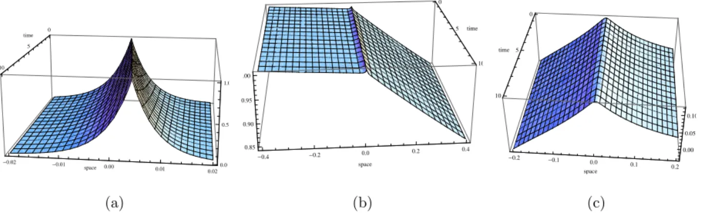
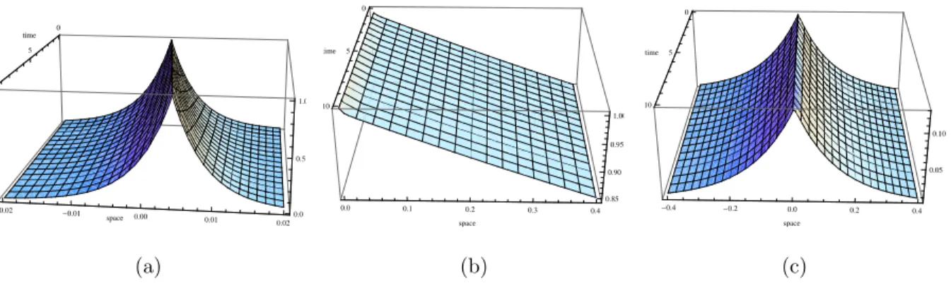
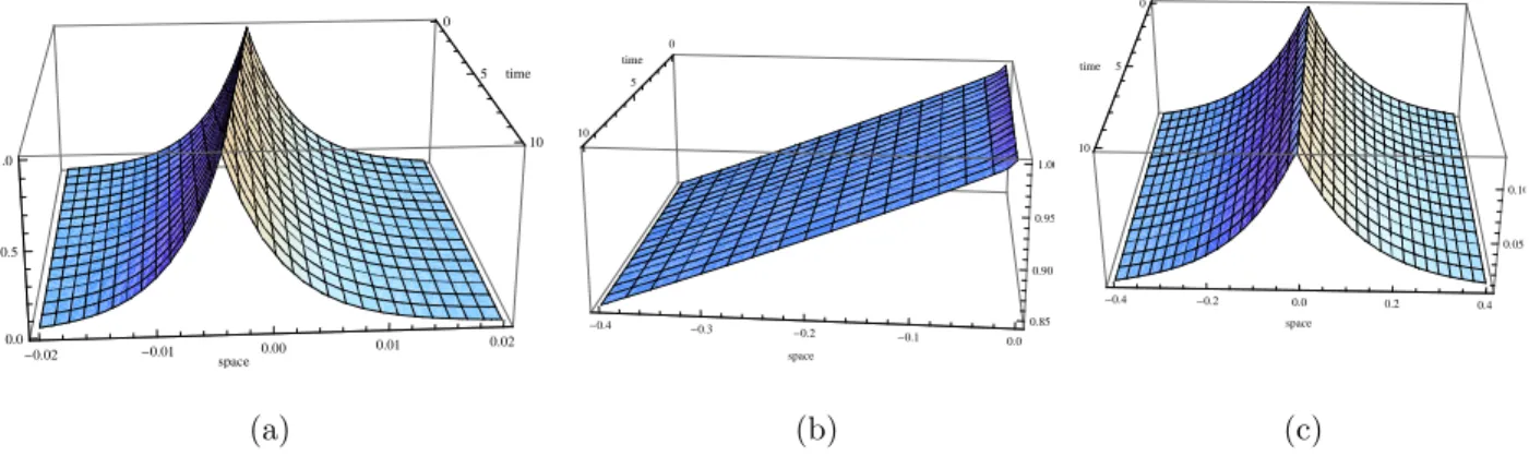
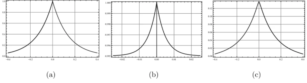
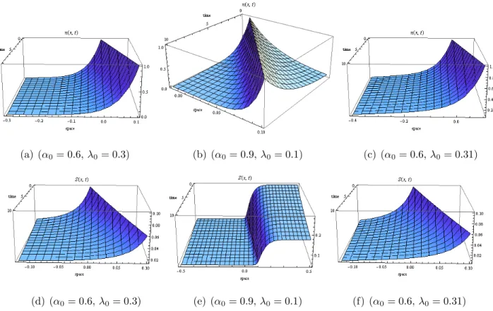
−(v_i²+k²_i)f_k_i(v_i) = 0. (2.30) Given that equation (2.26) is a nonhomogeneous second order differential equation (in q(u)) with constant coefficients, then the solutions q(u) are obtained after a direct integration of (2.26). We conduct our analysis with different values of a₂, and to display the behaviour of solutions we plot them in three dimensions, keeping the values of the parameters as set in the experiment as follows [111]: s = 10⁻²mm/sec, D_F = D_S = 10⁻³mm²/sec, α = β = 0.2/sec, γ = 0.05/sec, λ₀ = 1/sec, c = ±4.3 ×10⁻⁴mm/sec, p(0) = 1mM, and n₀ = λ₀N₀/s = 10³cells/cm³ = 1cell/mm³. The sub-figures (a) depict the distribution of the cells, while subfigures (b) and (c) depict the succinate and aspartate concentrations respectively. We note from the experiment that the α_i are very small (of order 10⁻²).

Assume 0< c < s

Theorem 2.3.1. When a₂ = 0, unique travelling wave solutions to (2.4)–(2.7) exist and are explicitly given by (2.28),

F(x, t) = p(u) =







p(0)e^−(c/(2D^F^))uI_k₁ α₁e^(σ¹^/2)u

/I_k₁(α₁), u <0, p(0)e^−(c/(2D^F^))uI_k₂ α₂e^−(σ²^/2)u

/I_k₂(α₂), u≥0,

(2.31)

(31)

0

5

10 time

-0.02 -0.01 space 0.00 0.01 0.020.0

0.5 1.0

(a)

5

10 time

-0.4 -0.2 0.0 0.2 0.4

space 0.85

0.90 0.95 1.00

(b)

0

5

10 time

-0.2 -0.1 0.0 0.1 0.2

space

0.00 0.05 0.10

(c)

Figure 2.1: Non starvation travelling waves in the case ofa2 = 0 andc > 0. Cells are very slowly distributed over the space (see subfigure (a)), and excrete a low concentration of aspartate with respect to the succinate (see subfigures (b) and (c)).

and

S(x, t) = q(u) =











γ₈e^−γ¹û+γ₉e^γ²û −αn₀p(0)e^−γ¹û γ₃I_k₁(α₁)

R0

u e^γ⁴^u¹I_k₁ α₁e^(σ¹^/2)u¹ du₁ +αn₀p(0)e^γ²^u

γ₃I_k₁(α₁) R0

u e^γ⁵^u¹Ik1 α1e^(σ¹^/2)u¹

du1, u <0, γ8e^−γ¹û+γ9e^γ²û +αn₀p(0)e^−γ¹û

γ₃I_k₂(α₂) Ru

0 e^γ⁶^u¹Ik2 α2e^−(σ²^/2)u¹ du1

− αn0p(0)e^γ²^u γ₃I_k₂(α₂)

Ru

0 e^γ⁷^u¹I_k₂ α₂e^−(σ²^/2)u¹

du₁, u≥0,

(2.32)

where u=x−ct,

γ₁ = (c+γ₃)/(2D_S), γ₂ = (γ₃−c)/(2D_S), γ₃ =p

c²+ 4γD_S, γ₄ =−c/(2D_F) +c/D_S+γ₂+σ₁, γ₅ =−c/(2D_F) +c/D_S−γ₁+σ₁, γ₆ =−c/(2D_F) +c/D_S+γ₂−σ₂, γ₇ =−c/(2D_F) +c/D_S−γ₁−σ₂, γ₈ = αn0p(0)(α1/2)^k¹

γ₃(γ₄+c/(2D_F))Γ(1 +k₁)I_k₁(α₁), γ₉ = −αn0p(0)(α2/2)^k²

γ₃(γ₇−c/(2D_F))Γ(1 +k₂)I_k₂(α₂), (2.33) and c is chosen so that

γ₂γ₉ ≤γ₁γ₈, γ₁ ≤ c

D_F +σ₂, γ₁γ₈e^σ¹^u ≤γ₂γ₉e^γ²^u, (2.34)

for any real u <0.

(Note that the proofs of all theorems are given in the Appendix.)

(32)

From the experiments, note that the constraint (2.34) is realistic. In fact, Budrene et al [13]

observed that the wave speedcis within the range 1−2mm/hour, and the diffusion coefficients are of order 10⁻⁵cm²/sec.

Now we assume a₂ 6= 0.

Theorem 2.3.2. When a₂ >0, non zero travelling wave solutions do not exist.

Theorem 2.3.3. For max (−c²/(4D_F),−γ)< a₂ < 0, travelling wave solutions exist and are given by (2.28),

F(x, t) =F(0,0)e^a²^tI_k₂ α₂e^−(σ²^/2)u

e^−(c/(2D^F^))u/I_k₂(α₂), u≥0, (2.35) and

S(x, t) = e^a²^tq(u), (2.36)

with

q(u) =











(1 +τ2/τ1)δ1e^τ²^u, u <0, τ₂δ₁

τ₁ e^−τ¹û+δ1e^τ²û+αn₀F(0,0)e^−τ¹û τ₃I_k₂(α₂)

Ru

0 e^τ⁴^u¹Ik2 α2e^−(σ²^/2)u¹ du1

−αn0F(0,0)e^τ²^u τ₃I_k₂(α₂)

Ru

0 e^τ⁵^u¹Ik2 α2e^−(σ²^/2)u¹

du1, u≥0,

(2.37)

where u=x−ct,

δ₁ = −αn₀F(0,0)(α₂/2)^k²

τ₃(−σ₂k₂/2 +τ₅)Γ(1 +k₂)I_k₂(α₂), τ₁ = (c+τ₃)/(2D_S), τ₂ = (−c+τ₃)/(2D_S), τ₃ =p

c²+ 4D_S(a₂ +γ), τ₄ =−c/(2D_F) +c/D_S+τ₂−σ₂,

τ5 =−c/(2DF) +c/DS−τ1−σ2, (2.38) and c is chosen so that τ₁ ≤σ₂k₂/2 +c/(2D_F) +σ₂, i.e.,

c+p

c²+ 4D_F(a₂+γ)

2D_S ≤ c+√

c²+ 4a2DF

2D_F + 2λ0

s−c. (2.39)

Likewise, we note from biological observations that (2.39) is a realistic constraint. The notation max(a, b) stands for the maximum value between a and b.

(33)

0

5

10 time

-0.02 -0.01 space 0.00 0.01 0.020.0

0.5 1.0

(a)

5

10 time

0.0 0.1 0.2 0.3 0.4

space

0.85 0.90 0.95 1.00

(b)

0

5

10 time

-0.4 -0.2 0.0 0.2 0.4

space

0.05 0.10

(c)

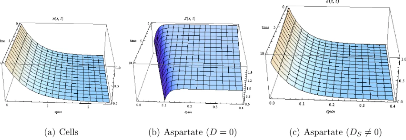
Figure 2.2: Non starvation travelling waves in the case where a₂ <0 and c >0 (a₂ =−10⁻⁵).

Theorem 2.3.4. For max(−c²/(4D_F),−γ) < a₂ <0, travelling wave solutions exist and are given by (2.28),

F(x, t) =







F(0,0)e^a²^tI_k₁ α₁e^(σ¹^/2)u

e^−(c/(2D^F^))u/I_k₁(α₁), α₀t≤x < ct, F(0,0)e^a²^tI_k₂ α₂e^−(σ²^/2)u

e^−(c/(2D^F^))u/I_k₂(α₂), x≥ct,

(2.40)

and

S(x, t) = e^a²^tq(u), (2.41)

with

q(u) =











δ₁₁e^−τ¹û+δ₁e^τ²û− αn0F(0,0)e^−τ¹û τ₃I_k₁(α₁)

R0

u e^τ⁶^u¹I_k₁ α₁e^(σ¹^/2)u¹ du₁ +αn0F(0,0)e^τ²^u

τ₃I_k₁(α₁) R0

u e^τ⁷^u¹I_k₁ α₁e^(σ¹^/2)u¹

du₁, u <0, δ₁₁e^−τ¹û+δ₁e^τ²û+ αn₀F(0,0)e^−τ¹û

τ₃I_k₂(α₂) Ru

0 e^τ⁴^u¹I_k₂ α₂e^−(σ²^/2)u¹ du₁

−αn₀F(0,0)e^τ²^u τ₃I_k₂(α₂)

Ru

0 e^τ⁵^u¹I_k₂ α₂e^−(σ²^/2)u¹

du₁, u≥0,

(2.42)

where u=x−ct, τ1, τ2, τ3, τ4, τ5 and δ1 are given in (2.38), τ41, τ51, δ11 and α0 by τ₆ =−c/(2D_F) +c/D_S +τ₂+σ₁, τ₇ =−c/(2D_F) +c/D_S−τ₁+σ₁ δ₁₁ = αn₀F(0,0)(α₁/2)^k¹