HYDROGEOLOGICAL CONCEPTUAL MODELING OF THE KOSI BAY LAKES SYSTEM, NORTH EASTERN SOUTH AFRICA
By
MBALI NDLOVU
Submitted in fulfilment of the academic requirements for the degree of Master of Science
In Hydrogeology
Discipline of Geological Science
College of Agriculture, Engineering and Science University of KwaZulu-Natal
Durban South Africa
December 2015
As the candidate’s supervisor I have/have not approved this thesis/dissertation for submission.
Signed: ________________ Name: __________________ Date: ________________
ii
PREFACE
The research reported in this dissertation was completed by the candidate while based in the Discipline of Geological Science, School of Agricultural, Earth and Environmental Sciences of the College of Agriculture, Engineering and Science, University of KwaZulu-Natal, Westville Campus, South Africa. The research was partially supported by the Water Research Commission and the University of KwaZulu-Natal.
The contents of this work have not been submitted in any form to another University. Except where the work of others is acknowledged in the text, the results reported are due to investigations by the candidate.
iii
DECLARATION 1: PLAGIARISM
I, Mbali Ndlovu, declare that:
i. The research reported in this dissertation, except where otherwise indicated or acknowledged, is my own original work;
ii. This dissertation has not been submitted in full or in part for any degree or examination to any other university;
iii. This dissertation does not contain other persons’ data, pictures, graphs or other information, unless specifically acknowledged as being sourced from other persons;
iv. This dissertation does not contain other persons’ writing, unless specifically acknowledged as being sourced from other researchers. Where other written sources have been quoted, then:
a. Their words have been re-written but the general information attributed to them has been referenced;
b. Where their exact words have been used, their writing has been placed inside quotation marks, and referenced;
v. Where I have used material for which publications followed, I have indicated in detail my role in the work;
vi. This dissertation is primarily a collection of material, prepared by myself, published as journal articles or presented as a poster and oral presentations at conferences. In some cases, additional material has been included;
vii. This dissertation does not contain text, graphics or tables copied and pasted from the Internet, unless specifically acknowledged, and the source being detailed in the dissertation and in the References sections.
______________________
Signed: Mbali Ndlovu Date: December 2015
iv
ABSTRACT
This M.Sc. Thesis focuses on the hydrogeological study of the Kosi Bay Lakes system, located in the north-eastern KwaZulu-Natal (KZN) Province of South Africa. The research catchment covers an area of about 659 km2. It is characterised by four interconnected lakes, two isolated lakes and an estuary with a combined area of about 48 km2. Two fresh water streams; namely, Sihadhla and Gezisa drain into the lakes. The study was initiated due to information gaps and the importance of the area with respect to conservation, ecology and water resources. The main objectives of the research was to characterize the groundwater and surface systems, in terms of their interconnection, flow and hydrochemistry; conduct a water balance study and develop a conceptual hydrogeological model on the occurrence and interaction of groundwater and surface water within the study area. The study has been undertaken by collecting primary data through a series of field campaigns in April 2013, May 2013 (onsite measurements and water, and water sampling) and October to December 2014 (geophysical data collection and supervision of borehole drilling). Original data generated in this study was complimented with data from KZN Groundwater Resource Information Project (GRIP), the National Groundwater Archives (NGA) and geophysical data, borehole logs, chemistry, and borehole yield data from consultant reports. Geophysical sounding data were calibrated using borehole logs and aquifer pumping tests, which indicate the presence of three hydrostratigraphic units in the study area, namely; the unconfined Holocene cover sands, the Kosi Bay and Port Durnford Formations, and the leaky-confined aquifer made up of the Umkhwelane and Uloa Formations, from top to bottom, respectively. The mean annual precipitation (MAP) for the study area based on data collected at Ingwavuma Kosi Bay and Ingwavuma Manguzi meteorological stations is 939 mm/year. The mean annual groundwater recharge estimated using the chloride mass balance method is 13% of the MAP. Surface water runoff from the catchment to the lakes derived using the Runoff Curve Number method is 14% of the MAP. Evaporation rate from the lakes and evapotranspiration from the catchment area estimated using the Penman and FAO Penman- Monteith approach are 1341 mm/a and 1135 mm/a, respectively. The water balance parameters indicate that inputs into the lakes are greater than the output as indicated by the positive change in storage (∆S). The lake water balance result was supported by long-term lake level records that show an increasing trend over time. The measured electrical conductivity (EC) for the Kosi Bay Lakes range from 1024 μS/cm (Amanzamnyama) to 24600 (Makhawulani) μS/cm, for the groundwater from 86 to 400 μS/cm and for the streams, it ranges from 227 to 341 μS/cm. The
v high EC and TDS values of some of the Kosi Bay Lakes are attributed to the high evaporation and connection to the sea through the estuary. The shallow aquifers are characterized by Na- HCO3-Cl, whereas the deep aquifers have a Na-Ca-Cl hydrochemical facies. All groundwater, stream and lake water samples have δ18O and δ2H values that plot on the local and global meteoric water lines indicating recharge from meteoric sources. Groundwater in the shallow Holocene aquifer and streams has similar hydrochemical and isotopic signature, indicating strong interconnection. On the other hand, the lakes are characterized by Na-Cl hydrochemical water type and an enriched stable isotopic signal (positive δD and δ18O signals) indicating evaporation and terminations of the local surface and groundwater flow system. The detectable tritium signal along with the low salinity of groundwater in the shallow aquifer reflect recent (< 50 years) recharge.
vi
ACKNOWLEDGMENTS
Firstly I would like to extend my sincere thanks to my supervisor Dr. Molla Demlie, thank you for the opportunity, for your guidance and for always pushing me throughout the research.
I wish to thank Mark Schapers, words could never describe how grateful I am for the field experience that I gained at Jeffares & Green (Pty) Ltd, thank you for the long and passionate talks about the coastal flats. Your kindness, patience and guidance is appreciated.
I wish to thank Jan Weitz, my fellow colleague. It has been a huge pleasure sharing an office with you. Thank you for our long talks and the time we spent venting, it kept me sane throughout the two years. I wish to thank Zesizwe Ngubane, for being a supportive and for making everything easy for me. It has been awesome getting to know you.
I wish to thank my family and friends, I can never thank you enough for your prayers, love, support and unconditional love throughout the years. To Vikani Funda, my pillar of strength, my blessing from day one. Thank you for standing right beside me always, for believing in me when I did not believe in myself and for being a best friend.
vii TABLE OF CONTENTS
Page
PREFACE ... ii
DECLARATION 1: PLAGIARISM ... iii
ABSTRACT ... iv
ACKNOWLEDGMENTS ... vi
LIST OF TABLES ... ix
LIST OF FIGURES ... xi
LIST OF ACRONYMS ... xiii
CHAPTER 1- INTRODUCTION ... 1
1.1 Background and Rationale ... 1
1.2 Research aims and objectives ... 2
1.3 Thesis structure ... 2
CHAPTER 2 –DISCRIPTION OF THE STUDY AREA ... 4
2.1 Location ... 4
2.2 Drainage and Physiography ... 5
2.3 Hydrometeorology and Climate ... 7
2.4 Land use and vegetation ... 8
2.5 Demography and economic activities ... 9
2.6 General geological and hydrogeological settings ... 10
2.7 Coastal evolution ... 14
CHAPTER 3- LITERATURE REVIEW ... 16
3.1 Conceptual modelling ... 16
3.2 Application of geophysical methods in hydrogeology ... 19
3.3 Water balance ... 23
3.4 Analysis and modelling of groundwater-surface water interactions ... 29
3.5 Previous Studies on Lake –groundwater interactions ... 32
CHAPTER 4-METHODOLOGY AND MATERIAL ... 34
4.1 Desktop studies ... 34
4.2 Fieldwork ... 34
4.3 Laboratory work ... 35
4.4 Statistical analysis of hydrochemical data ... 38
viii
4.5 Water balance ... 39
4.6 Groundwater recharge ... 40
4.7 Runoff from the catchment ... 40
4.8 Evaporation from the Lakes ... 42
4.9 Evapotranspiration from the catchment ... 43
4.10 Groundwater and surface water abstraction ... 44
4.11 Groundwater seepage/outflow to the Indian Ocean ... 45
4.12 Gephysical incestigation ... 46
4.13 Delineation of Wetlands and Lakes Capture Zone ... 47
4.14 Data analysis tools ... 48
CHAPTER 5-RESULTS AND DISCUSSION ... 50
5.1 Results of Geophysical investigation and borehole drilling ... 50
5.2 Aquifer Classification and their hydraulic properties ... 54
5.3 Groundwater recharge, local groundwater flow direction and groundwater contributing area ... 55
5.4 Wetland Capture zone delineation ... 58
5.5 Water balance analysis ... 60
5.6 Hydrochemistry ... 63
5.7 Statistical analysis of hydrochemical data ... 68
5.8 Environmental isotopes (δ2H, δ18O and 3H) ... 71
5.9 Water resource quality in the Kosi Bay Lakes catchment ... 74
5.10 Hydrogeological conceptualization of the Kosi Bay Lakes catchment ... 76
CHAPTER 6- CONCLUSIONS AND RECOMMENDATIONS ... 79
REFERENCES ... 82
APPENDICES ... 91
ix
LIST OF TABLES
Table Page
Table 2.1: Meteorological data (SAWS, 2014). ... 8 Table 3.1: Correlation of the biostratigraphic, Lithostratigraphic and geoelectrical subdivision
of the Cenozoic and late Mesozoic succession on the Zululand Coastal Plain (Meyer et al., 2001). ... 21 Table 4.1: Land use properties ... 42 Table 4.2 Annual surface water and groundwater abstraction within the Kosi Bay catchment
(DWAF, 2015). ... 44 Table 4.3: Groundwater abstraction estimation. ... 45 Table 5.1: Vertical Electrical Sounding (VES) inversion results found based on the
Schlumberger array. ... 52 Table 5.2: Summary of Hydraulic properties of aquifer layers underlying the Kosi Bay area..
... 55 Table 5.3: Point groundwater recharge estimation using the chloride mass balane method within
the study area ... 56 Table 5.4: Long term monthly estimated major water Lake balance components (in 106 m3)..
... 61 Table 5.5: Long term mean annual lake water balance of the Kosi Bay Lake (in 106 m3). ... 61 Table 5.6: Mean monthly estimated catchment's volumetric water balance components (in 106 m3). ... 63 Table 5.7: Annual catchment water balance of the Kosi Bay Lake (106 m3). ... 63 Table 5.8: Pearson’s correlation matrices for groundwater data. All values in mg/l unless
otherwise indicated. ... 69 Table 5.9: Results of principal component factor analysis with Varimax rotation of groundwater
data. All values in mg/l unless otherwise indicated. ... 70
x Table 5.10: South African Water Quality guidelines for domestic, industrial and agricultural use (SAWQ, 1996) and World Health Organization guidelines for drinking water (WHO, 2011). ... 76
xi
LIST OF FIGURES
Figure Page
Figure 2.1: Location map of Kosi Bay lakes system... 4
Figure 2.2: Local surface water drainage and physiography of the Kosi Bay area. ... 6
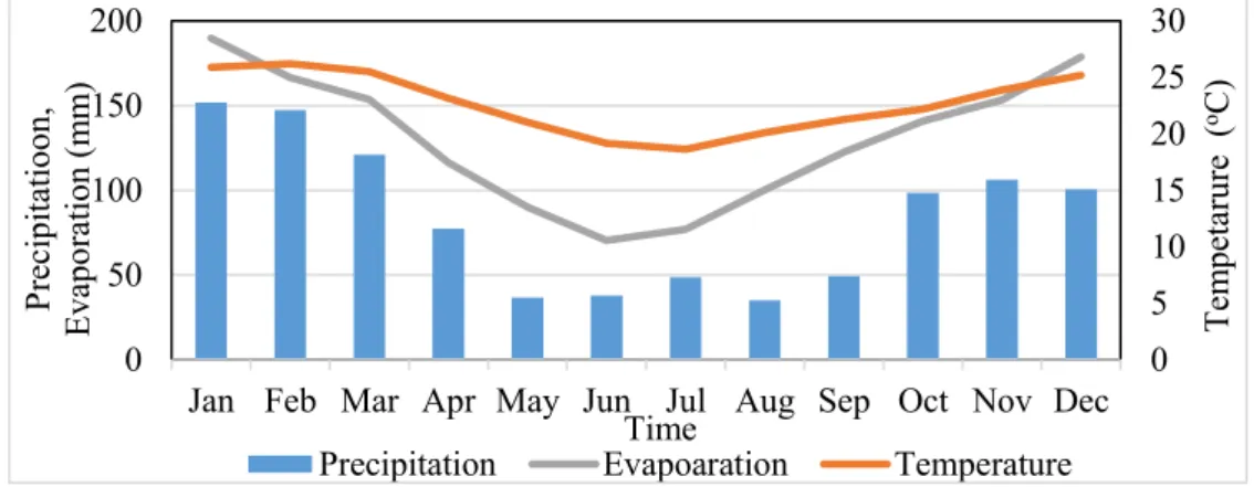
Figure 2.3: Mean monthly rainfall data from Ingwavuma Kosi Bay station, mean monthly temperature data from Mbazwana station and W7 catchment S pan evaporation (SAWS, 2014). ... 7
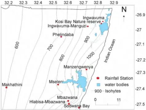
Figure 2.4: Spatial distribution of annual rainfall for the area around the Kosi Bay Lakes system. ... 8
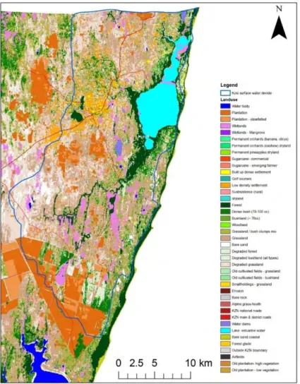
Figure 2.5: Land cover map of the north eastern KZN Land cover map of the north eastern KZN (modified) (SANBI, 2016).. ... 9
Figure 2.6: Geological Map of north-eastern KwaZulu-Natal (modified from Porat & Botha, 2008). ... 11
Figure 2.7: A schematic geological cross section of the northern KwaZulu-Natal coastal plain (not to scale), Bruton and Cooper (1980)………...12
Figure 3.1: Histogram of surface measured formation resistivities based on calibrations soundings (Worthington, 1978). ... 20
Figure 3.2: Comparison between the results of time domain electromagnetic sounding interpretations (TDEM) and drilling results (modified from Mayer et al., 2001)……… 22
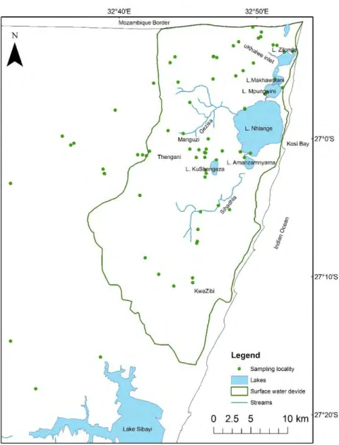
Figure 4.1: The location of groundwater and surface water sampling points within and around the study catchment………..36
Figure 4.2: Photographs of the borehole samples collected for logging. ... 37
Figure 4.3: A typical Schlumberger array ... 46
Figure 5.1: Spatial distribution of the location of geophysical investigation sites. ... 51
xii Figure 5.2: Well to well geological cross-section in the Kosi Bay catchment. ... 53 Figure 5.3: Spatial distribution of groundwater recharge within the Kosi Bay catchment using
CMB method ... 57 Figure 5.4: Local groundwater flow direction map, with a delineated groundwater boundary (593 km2) illustrating water that contributes to the overall water balance. ... 58 Figure 5.5: Capture zone delineated using the hydrogeological mapping method at a wetlands.
... 59 Figure 5.6: Long term lake level changes with monthly precipitation from 1977- 2014 (lake
level data from DWA, 2015 and Precipitation data from SAWS, 2014). ... 62 Figure 5.7: (a) Trilinear piper and (b) Schoeller diagram of groundwater and surface samples
of April 2013, in and around Kosi Bay Lake Catchment. ... 66 Figure 5.8: (a) Trilinear piper and (b) Schoeller diagram of groundwater sample showing
chemical composition, dating from 2005-2014, in and around Kosi Bay Lake Catchment. ... 67 Figure 5.9: Results of principal component analysis in rotated space of the groundwater
chemistry data ... 71 Figure 5.10: Plot of δ18O and δ2H of water samples collected within the Kosi Bay catchment
along with the Local and Global meteoric water lines. ... 72 Figure 5.11: 18-Oxygen versus Deuterium cross plot for the surface water samples along with
the Local and Global meteoric water lines. ... 73 Figure 5.12: 18-Oxygen versus Deuterium cross plot for the Kosi Bay catchment groundwater
samples along with the Local and Global meteoric water lines. ... 74 Figure 5.13: Hydrogeological conceptual model of the Kosi Bay catchment. ... 78
xiii
LIST OF ACRONYMS
C Runoff coefficient
Clp Chloride concentration in precipitation [mg/l]
Clgw Chloride concentration in groundwater [mg/l]
CMB Chloride mass balance
CN Curve Number
DEM Digital elevation model
R Recharge [mm/year]
DO Dissolved oxygen [ppm]
DWA Department of Water Affairs DTWL Depth to water-level [m.bgl]
EC Electrical conductivity [mS/m]
Eh Reduction potential [mV]
FAO Food and agriculture organisation GMWL Global meteoric water-line IC Ion chromatograph
ICP-MS Inductively coupled mass spectrometry LMWL Local meteoric water-line
m3/a Cubic meter per annum MAP Mean annual precipitation MCM/a Million cubic meter per annum ORP Oxygen reduction potential [mV]
P Precipitation [mm/month]
RH Relative humidity [%]
SAR Sodium adsorption ratio SAWS South African weather service TDEM Time domain electromagnetic TAL Total alkalinity [mg/l]
TDS Total dissolved solids [ppm]
TU Tritium unit
UNESCO United Nations Educational, Scientific and Cultural Organization WMA Water Management Area
1
CHAPTER 1- INTRODUCTION
1.1 Background and RationaleSouth Africa is a semi-arid country characterized by low average rainfall with a growing population which may pose a great challenge in the provision of water supply for domestic, agricultural and industrial purposes. In this regard, water in South Africa should be treated as a very important natural resource that needs to be preserved and protected for the current and future generations. Surface water has been the main focus in both development and exploitation in most parts of South Africa over the years with the exception of rural areas such as northern KwaZulu-Natal where groundwater remains the main source of water for the rural communities (Bredenkamp et al., 1995,Mayer and Godfrey, 1995, Kelbe et al., 2001). The Kosi Bay Lake System, which is the focus of this study, is one of the most pristine Lake systems on the South African coast and has been used for recreational fishing since the 1950s (James et al., 2001). It is an ecologically important wetland system that falls within the ISimangaliso Wetland Park and has been designated as one of the registered RAMSAR Convention Wetlands of International Importance (RAMSAR Site no.527; UNESCO, 2015). The Kosi Bay Lakes system is a complex, interconnected and dynamic hydrological system made up of interconnected groundwater, stream, lakes, wetlands and estuary system. These interconnections mean that a change in one element of the system may have serious implications on the entire hydro-ecosystem. Local communities that reside in the western part of the catchment are largely dependent on groundwater for their water supply.
Historically, there have been several studies conducted along the coastal plain. Significant to the current research includes works done by Worthington, 1978; Mayer et al., 1982; Mayer and Godfrey, 1995; Wright et al., 2000; Kelbe et al.,2001; Mayer et al., 2001; Wright, 2002; Porat and Botha, 2008; Kelbe and Germishuyse, 2010 and Weitz and Demlie, 2014. A review of these and other literature in the area revealed that detailed information regarding the hydrogeology, hydrochemistry, the rate of groundwater abstraction in the catchment and its impact on the lakes, the overall water balance of the Lakes system and the interaction of the various hydrological elements within the Lakes Kosi Bay catchment remain poorly understood. Thus, in order to overcome this information gap on one of the most pristine Lake system on the South
2 African Coast, it is vital that the hydrogeological characteristics of both groundwater and surface water is understood, all the water balance components of the Lake system be quantified and interaction of lake–groundwater understood and available to the decision makers.
1.2 Research aims and objectives
This dissertation aims to contribute towards improved understanding of the hydrological functioning of the Kosi Bay Lakes catchment including the interaction of surface water and groundwater by collecting and integrating hydrogeological data.
The main objectives of the research are:
a) To characterize groundwater and surface water in terms of interconnection, flow and hydrochemistry.
b) To undertake a water balance analysis of the Lakes system including its catchment.
c) To develop a conceptual hydrogeological model for the Kosi Bay Lakes catchment that explains among others the interaction between surface water and groundwater.
1.3 Thesis structure
Chapter one set out the background and rational to the research and introduces to the scope, aim and objective of the research.
Chapter two presents a systematic description of the study area by providing the most important salient features such as the geology in terms of stratigraphy and, lithology general hydrology and hydrogeology, climate, land use - land cover, coastal evolution and the likes.
Chapter three provides a literature review which outlines and discusses the state of the science of the catchment and lake water balances, and conceptual modelling of the interaction of surface water and groundwater
Chapter four outlines the methods and the material used in the study to collect, analyse and interpret the data generated.
Chapter five focusses on the results obtained, outlining and discussing the
3 hydrogeological unit, groundwater recharge and flow direction, lake and catchment water balance, hydrochemical and environmental isotope results, water quality, the conceptual modelling of the Kosi Bay lakes system.
Chapter six draws conclusions and provides recommendations for future research.
References used and cited within the text and appendices are presented after the conclusion.
4
CHAPTER 2 –DISCRIPTION OF THE STUDY AREA
2.1 LocationThe Kosi Bay Lakes system is made up of four interconnected lakes, two isolated lakes and an estuary (Figure 2.1). The Lakes system is located along the northeastern coastal region of South Africa which is part of the largest primary aquifer system that stretches from Mtunzini in the south up to the Mozambique border in the north (Mayer et al., 2001).
The catchment area is estimated to be about 659 km2 of which 48 km2 is covered by the lakes and estuary. These Lakes are Makhawulani (0.117 km2), Mpungwini (3.299 km2), Nhlange (38.853 km2) and Amanzamnyama (1.860 km2), from north to the south, respectively and are connected to the Indian Ocean through the Kosi mouth (estuary).
Gezisa and Sihadhla are the two main perennial streams that drain into the lakes.
Figure 2.1: Location map of Kosi Bay lakes system.
5 2.2 Drainage and Physiography
The Kosi Bay Lakes System is situated on the Zululand coastal plain. It is made up of 4 interconnected lakes that are linked to the sea by a single outlet called the Kosi mouth (estuary). The Kosi Bay Lakes system has a north-south orientation and drains to the Indian Ocean. The limit of the lake’s catchment was defined using a Digital elevation model (DEM) and it is constrained by the coastal dune cordon in the east and the older dunes in the west. The deepest lake is Nhlange (32 m), followed by Mpungwini (21 m), Makhawulani (8 m) and Amanzamnyama (2 m) (Wright, 2001). It is through the Kosi mouth that the salt water inters the system, while the fresh water is thought to enter through groundwater and small streams around the Lakes. Hence, the existence of a salinity gradient from fresh conditions at Lake Amanzamnyama in the south to saline conditions in the Kosi mouth (Mayer et al., 2001; Ndlovu and Demlie, 2015). The Lakes system except the Kosi mouth is secluded from the ocean by densely forested sand dunes that are as high as 130 m a.m.s.l (Wright, 2002). While on the western side, it is bound by paleodune cordons, which demarcates the western catchment boundary of the lakes (Figure 2.2). The coastal parabolic dunes are important features of the Kosi Bay area and are described in detail in Porat and Botha (2008). These coastal dunes are made up of the Sibayi Formation and are known to trend in an approximate north-south direction along the coast.
The area characterized by flat topography, permeable sands, wetlands and flood plains of Gezisa and Sihadhla streams flowing towards Lake Nhlange and Lake Amanzamnyama, respectively (Figure 2.2). The elevation of the area varies from zero meters above mean sea level (a.m.s.l) to about 102 m a.m.s.l further inland. The two streams are perennial and drain across the wetlands, which is typical of coastal water bodies. The Sihadhla stream is associated with peat soilsfrom the swamp forest vegetation and is very nutrient poor (Begg, 1978; Grobler et al., 2004), hence the association of Lake Amanzamnyama with the dark colored organic material.
The swamp forest wetland is a major feature of the Kosi Bay area. It is part of the ISimangaliso wetland park, which has been designated as a Ramsar site (Site No.527) of
6 international importance. The wetlands found in the Maputaland coastal plain are situated in low lying interdune, valley bottom areas and underlain by low permeability sediments and cover most of the Kosi Bay area and extends further on the western side (SANBI, 2014). Worthington (1978) reported that the underlying aquifers are fully saturated from the surface of Cretaceous basement up to the shallow water table. According to Rawlins and Kelbe (1998) and Grundling et al. (2013), there has been a decrease in the water levels around the area over the past years. This is evident through drying of hand operated shallow boreholes and pans. Since the wetlands within the area are directly linked to groundwater and surface water, and are highly dependent on climatic changes and land use, this becomes a challenge. Rawlins and Kelbe (1998) established that the increased agricultural activities together with forestry and rural water supply schemes on the Maputaland coastal plain are the main reasons behind the decrease in the level of groundwater resources. Wetlands are nutrient rich and water saturated in nature, therefore, are used by the local community for subsistence farming, plantation and forestry.
Figure 2.2: Local surface water drainage and physiography of the Kosi Bay area.
7 2.3 Hydrometeorology and Climate
The general climate of the area can be described as humid subtropical with warm summers, dominated by southern subtropical high pressure belt (Hunter, 1988, Wright, 2002). Pan evaporation data retrieved from the Department of Water Affairs and Sanitation (DWA, 2014) for the Kosi Bay Lakes catchment is about 1450 mm/a. Rainfall occurs throughout the year along the coast, but a large portion of it is experienced mostly in the summer months (Figure 2.3).
Figure 2.3: Mean monthly rainfall data from Ingwavuma Kosi Bay station, mean monthly temperature data from Mbazwana station and W7 catchment S pan
evaporation (SAWS, 2014).
The rainfall varies from 1100 mm/year along the coast and decreases towards the west to less than 600 mm/year at the base of the Lebombo Mountain range (Figure 2.4). Kelbe et al. (2001) reported that the rate of groundwater recharge and surface runoff in northeastern region of KwaZulu-Natal is controlled directly by rainfall more than any other catchment factors. January experiences the highest evaporation rate. Temperature records from the Mbazwana Airfield meteorological station indicates a mean temperature of 22.6 °C (varying from 18.6 °C in July to 26.2 °C in February). Relative humidity ranges between 80.4 % in December to 91.2 % in July (Table 2.1).
0 5 10 15 20 25 30
0 50 100 150 200
Jan Feb Mar Apr May Jun Jul Aug Sep Oct Nov Dec
Tempetarure (oC) Precipitatioon, Evaporation (mm)
Time
Precipitation Evapoaration Temperature
8 Figure 2.4 Spatial distribution of annual rainfall for the area around the Kosi Bay Lakes
system (rainfall data from SAWS).
Table 2.1: Meteorological data from various stations (SAWS, 2014).
Jan Feb Mar Apr May Jun Jul Aug Sep Oct Nov Dec Rainfall 135.96 132.29 113.78 68.48 28.30 38.25 34.89 28.42 45.54 86.90 109.46 107.02 Temperature
(°C) 25.88 26.21 25.49 23.15 21.04 19.15 18.64 20.11 21.28 22.19 23.87 25.19 Humidity
(%) 82.80 84.63 87.27 89.64 89.33 91.13 91.20 87.27 83.00 81.67 80.53 80.40 Wind speed
(m/s) 2.55 2.55 2.55 2.55 2.55 1.52 1.76 2.16 2.67 2.94 3.03 2.85 Pan evaporation 189.76 166.54 153.48 116.23 90.16 70.47 76.90 100.35 122.52 140.78 153.30 178.72 Sunshine
duration (hours)
6.63 6.96 7.17 7.19 7.61 6.71 7.26 7.63 6.65 5.66 5.68 6.14
2.4 Land use and vegetation
Because of the limited occurrence of mineral deposits, the study area can be classed as underdeveloped as far as mining activities are concerned. The same is true for agricultural activities. These resulted in limited infrastructure development (Watkeys et al., 1993).
Hence the Kosi Bay Lakes system still remains by far the most pristine lake system on the South African coast. The extensive redistribution of the nutrient poor sandy soil limits the utilization of the readily available land for agricultural purposes. This has also
9 contributed to the preservation of the area’s ecosystem. Looking at the land cover map (Figure 2.5), greater than 10 percent of the land is covered by water bodies and wetlands.
Grassland and cultivated land are the most dominant land covers, while the urban areas cover a small proportion of the catchment.
Figure 2.5: Land cover map of the north eastern KZN (modified) (SANBI, 2016).
2.5 Demography and economic activities
The Kosi Bay Catchment falls within uMhlabuyalingana local Municipality which is one of the five municipalities under uMkhanyakude District. The towns within the catchment are Manguzi and Thengani. UMhlabuyalingana Municipality has a population of about 156 736 people and the majority resides in deep rural, traditional authority areas (Stats SA, 2012). Kosi Bay is under the W70A Quaternary catchment which falls under the
10 Usuthu-Mhlatuze Water Management Area (WMA), and the local communities depend on groundwater for their supply (DWAF, 2008).
Apart from private groundwater abstraction through hand operated boreholes by the local community, the Inkanyezini and Kwangwanase water supply schemes pump and supplies water from more than 10 production boreholes to the local communities in and around Manguzi to meet the water demand. The two schemes were implemented in the 1990’s and have since been in operation until present. The scheme supplies water to an estimated population of about 73 000 people at 60 liters per person per day, and the number is expected to increase (Holliday, 2012). Additional raw surface water is abstracted from Gezisa and Nkanini streams, and Shengeza Lake (Jeffares & Green, 2008). In addition to the Kwangwanase and Inkanyezini schemes, the Mbazwana, Mpophomeni-Mseleni, Phelindaba, Shemula, Mbila, Qondele-Gujini and KwaZibi water supply schemes supply the north eastern part of the UMkhanyakude District Municipality (Stats SA, 2012).
2.6 General geological and hydrogeological settings
2.6.1 Geology
Geologically, North-eastern KwaZulu-Natal Province is underlain by Mesozoic and Cenozoic sediments (Figure 2.6 & 2.7). The Cretaceous age deposits of the Zululand Group comprising of the Makhathini, Mzinene and St Lucia Formations from bottom to top, respectively, are the lower most layers underlying the north KwaZulu-Natal, at least from a hydrogeological perspective. These Zululand Group sediments are overlain by the Maputaland group sediments, these sediments are mostly infertile, wind-blown distributed sands. The Maputaland comprises of the late Miocene Uloa Formation, which in turn overlain by the early Pliocene cross-bedded calcarenites of the Umkhwelane Formation (Mayer et al., 2001).
The Umkhwelane Formation is overlain by the loosely consolidated sands, silts and clays of the Pleistocene age Port Durnford and Kosi Bay Formations. Overlying the Kosi Bay Formation are the redistributed dune sands of the KwaMbonambi Formation, which are
11 in turn overlain by the Holocene age sediments of the Sibayi Formation forming the cover sands and active dunes (Wright, 2002; Porat and Botha, 2008).
Figure 2.6: Geological Map of the north eastern KwaZulu-Natal (modified Porat and Botha, 2008).
12 Figure 2.7: A schematic geological cross section across the northern KwaZulu-Natal
Coastal plain (Bruton and Cooper, 1980).
2.6.2 Hydrogeology
The north eastern region of KwaZulu-Natal is primarily underlain by Quaternary sand deposits making up the largest primary aquifer in the Southern Africa (Mayer et al., 2001). Governing the primary aquifer are geological features and hydrogeological boundaries. The Kosi Bay Lakes catchment is complex and sensitive to anthropogenic stresses and the primary aquifer is directly linked to the water bodies within the system (Kelbe et al., 2001; Weitz and Demlie, 2014; Ndlovu and Demlie, 2015).
The hydrogeological classification of the area described by the DWAF (1998) in the published 1:500 000 “Hydrogeological Map Series of the Republic of South Africa, is
“a3”, which indicates that the principal groundwater occurrence is within intergranular aquifers that have yield range between 0.5 and 2.0 l/s. Groundwater quality contoured in the hydrogeological map suggests that the Electrical Conductivity (EC) to be in the range of 0 to 70 mS/m. Generally, drilling experience in the unconsolidated sands indicate that they are good aquifers as long as medium to coarse grained sands are encountered below the water table.
The St Lucia Formation is considered as the “hydrogeological basement” in north-eastern KwaZulu-Natal, dominated by a uniform fine siltstone with thin bands of hard sandy limestone and sandstone in some areas. This unit is considered as having low permeability, poor quality and quantity of groundwater with TDS > 8 000 mg/l (Mayer et
13 al., 2001). The coquina layer is yellowish brown, hard, coarse and characterized by shell fragments, while the Umkhwelane Formation is made up of coarse light grey sandy limestone.
The Uloa Formation is very important in hydrogeology as it can be regarded as one of the main aquifers in the stratigraphic sequence (Worthington, 1978). According to Mayer et al. (2001), it is possible that the upper layer of this coquina has been exposed to karst solution or chemical weathering before the deposition of the overlying layer.
The Port Durnford Formation overlies the Uloa Formation. It is relatively thick and made up of loosely consolidated sand, clays, silts and lignite. According to Mayer et al. (2001), the Port Durnford Formation is found along the entire coastal dune cordon; reaching 25- 30 m in thickness at the coast (Worthington, 1978) and is the most promising aquifer (Mayer et al., 2001). The layer is then divided into the lower argillaceous member, characterized by blue–grey sand and mudstones, overlain by thin yellowish brown sand and reddish shelly fragmented sandstone.
The upper arenaceous member of the Port Durnford Formation is the Kosi Bay Formation, it is about 15 m thick and predominated by aeolian facies with large scale cross-bedding and these are generally white, yellow or yellowish–orange in colour and are mostly fine grained (Worthington, 1978). Discontinuous thin beds of carbonaceous sand and lignite occur at various levels (Jeffares & Green, 2012).
The upper most part of Port Durnford Formation and the overlying Holocene sands are extremely difficult to distinguish because of the westward grading of the units and for this reason the western limit of the Formation could not properly be defined (Mayer et al., 2001).
The overlying aeolian and fluvial sands of middle to upper Pleistocene and Holocene age are dominated by fine grained sand and about 5% silt and clay (Mayer et al., 2001) and are largely unconsolidated. Inland, these sands are exposed and are called the Berea type
14 red sands. The vulnerability of the primary aquifer is high, mainly due to the unconsolidated and shallow nature of the aquifers in the coastal flats.
2.7 Coastal evolution
Coastal evolution as described by Wright (2002) is the product of the morphodynamic processes that arise in response to changes in external conditions. Studying coastal evolution helps to understand how the coastal plain and all its features were formed. It is an inevitable fact that human growth and existence always had and will continue to have an effect on the natural settings as a result, over the past 50 years, human activities have had an influence on the evolution of the coast.
The Northern KwaZulu-Natal coastal plain is associated with dune cordons from the Tertiary age in the west and progressively become younger toward the coast. These linear relic cordons are believed to have been formed adjacent to old coastlines, and dating them can reveal the past climate and sea levels influence on the evolution of the coast (Wright et al., 2000).
According to Wright et al. (2000), the areas best to observe the modern evolution of the coast along the Northern KwaZulu-Natal are areas such as the Lake Sibayi, Lake St Lucia and Kosi Bay Lakes system where all the historical data are repositioned. However, the lack of outcrops and fossil remains and the reworking of older sand that forms the cover still present a problem in understanding the Cenozoic evolution of the Northern KwaZulu- Natal coastal plain.
The Kosi Bay Lake system is one of the three large coastal water bodies in the northern KwaZulu-Natal formed as a result of the Mio-Pliocene low sea-level still stands (Wright, 2002). According to Wright et al. (2000), the still stands allowed the rivers to scour the channels into the underlying sedimentary sequence. In the quest for unravelling the historical settings of the area, Cooper et.al. (1989) reported Molluscan assemblages around Lake Nhlange, which are indications of tidal flats that had been in place a number of times where the lake is currently situated. The oldest tidal flat owes its existence to the
15 last interglacial. The 6-8 m terraces preserved west of the lake is evidence that the Last Glacial Maximum (sea level dropped to -130 m) had no effect on the terraces through river incision (Wright, 2002).
16
CHAPTER 3- LITERATURE REVIEW
Groundwater exploitation in the past decade has been heavily debated, mainly because of the increasing scarce water resources and the need to optimise its use in the African continent (Robin et al., 2006). Over and above, the basic principles are all available to the hydrogeological sector when it comes to predicting or anticipating the likely outcome of groundwater exploitation. Conventional hydrogeological studies and groundwater flow modelling are the principal tools that aid in groundwater investigations. However these methods are limited by information gaps in the geometry and hydraulic properties of the underlying aquifers and related data. Methods of determining aquifer properties include the analysis of borehole logs, the assessment of the aquifers response to pumping, hydrochemical and isotope data. This information and data assist in the development of conceptual hydrogeological model of the study area which can be used for various purposes independently or converted to a numerical groundwater flow model.
3.1 Conceptual modelling
A conceptual model is a simple method of representing why and how a hydrological system behaves in a particular way and is an effective way of representing the interaction between groundwater and surface across all landscapes. It is mainly based on the present situation of a system and cannot fully represent and describe the tiniest details of the flow system (Fetter, 2001). It serves as the most simplified way of representing field problems so that they can be analyzed. A hydrogeological conceptual model incorporates geological, hydrogeological and hydrochemical data into a model. A model depending on the purpose can be either of the following categories (Anderson and Woessner, 1992):
Predictive models: - these are models that can be used to predict what might occur or result in the long run.
Interpretative models: - these are models used for evaluating dynamics within the system.
Generic models: - these are models used to analyze hypothetical hydrogeological systems.
17 Conceptual models are often used to build numerical models for predictions, and are used mostly by managers for more informed decision making on groundwater use and management. The accuracy of conceptual models influence the quality of the result of a numerical model.
Conceptual models need a lot of data; the more the data used, the more reliable the model will be. The data needs to be updated as new data are available for the purpose of improving and increasing the confidence level on the proposed model. Data can be in the form of field maps, borehole logs, geophysical investigation results, pumping test, hydrochemical, and environmental isotope data. The resulting conceptual model is then used to define hydrological boundaries, aquifer units, water level and flow direction and hydrochemical evolution process of the system.
Defining hydrostratigraphic units is mostly challenging, especially in areas where the geology is very difficult to distinguish. Yet it still remains one of the most important tasks to do when constructing a conceptual model. Hydrostratigraphic units are defined and differentiated based on their geological properties on geological maps, borehole log and geophysical data. Borehole logs are a true reflection of what the layers on the ground look like, adding certainty to what is portrayed on geological maps, whilst geophysical results add to meaningful results, as it provides an estimate of the resistivity, depth and thickness of a geological layers, which in most cases must correspond to the borehole logs.
The Kosi Bay area is mainly composed of sands of different composition and age.
Hydrologically, they are defined based on their hydraulic properties such as storativity, transmissivity, hydraulic conductivity and specific yield that are obtained from pump test data. Hydrochemical data also aids in distinguishing between the hydrochemical characteristics of aquifer units.
Hydrostratigraphic unit boundaries are defined and spatially represented using maps. This is where the use of numerical interpolation and extrapolation methods are mostly needed.
The common interpolation techniques such as kriging, spline, and nearest neighborhood interpolation are nowadays easily available in most computer programs and software such
18 as GIS and Surfer. Kriging interpolation interpolates a probability surface that fits best to a scattered set of point values in two-dimensional space, it can be used in small area where sampling is systematic and assumes a uniform pattern of distribution of point values (Esri, 2016). Spline interpolation estimates values using a mathematical function that minimizes overall surface curvature, therefore, used to smooth out the effects on data. This method is best for gradually varying surfaces such as elevations, water-table depths, or pollution concentrations. It is not appropriate when there are large changes within a short horizontal Distance because it can overshoot estimated values (Esri, 2016). Nearest neighbourhood interpolation delaunay triangulation of the input points and selects the closest nodes that form a convex hull around the interpolation point, then weights their values by proportionate area (Esri, 2016), it is good for random sampling. Sometimes, areas where a large portion has limited data or there is no datum at all, the above techniques are applicable together with relevant assumptions.
In the current study area for instance, a map of the aquifer basement was created by adding the modified bathymetric surface of deep lakes and rivers in the area and assumed the depth for the areas with no data using the known geological data from surface contours, borehole logs and cross sectional transects done for the region (Kelbe and Germishuyse, 2010).
There are other approaches that can be used to create these maps, which include using literature in the form of scientific journals and reports, using deep coastal lake bathymetry and information about the palaeochennels and other geological features that can define the upper and the lower limits on the elevation of the surfaces. For the Maputaland basement, various literatures such as King (1972) and Meyer et al. (2001) described the basement surface as dipping at an angle of 3-5 degrees. Kelbe and Germishuyse (2010) used the palaeochennels proposed by Worthington (1978), Maud (1968) and Davies Lynn and Partners (1992) to develop a conceptual model and maps of the subsurface layers.\
19 3.2 Application of geophysical methods in hydrogeology
There are a number of geophysical methods used for a broad spectrum of purposes. For the purpose of mapping and investigating the occurrence of groundwater in an area covered by unconsolidated material, the electrical resistivity technique is the most suitable and cost effective geophysical technique, and allows a relatively rapid survey of the geological succession (Worthington, 1978). In the Zululand coastal plain, the electrical resistivity technique has shown that the contrast in resistivity and low resistance, depth of penetration capabilities and the speed of operation (Van Zilj, 1971;
Australian Groundwater Consultants, 1975; Worthington, 1978; Meyer and De Beer, 1981; Meyer et al., 1983; Meyer et al., 1987; Coetsee, 1991). The two techniques that have been successfully used in the coastal flats are direct current and the electromagnetic sounding techniques. The gravity method has been applied without success by the Directorate Geohydrology, DWAF in order to locate palaeo-channels in the area around St Lucia that are believed to have been infilled by the younger sediments. Two profiles were investigated and none of them showed the paleo-channels that were identified by the drilling operation, resulting in the abandonment of the technique.
Worthington (1978) and Meyer et al. (2001) conducted a detailed geophysical work in the Zululand coastal plain using the Schlumberger technique. Despite the fact that the sounding curves were calibrated using existing nearby boreholes, the interpretation proved to be very difficult especially because of the homogenous nature of the coastal sands. Worthington (1978) analysed 900 sounding curves to establish the geological succession above the impermeable Cretaceous and Palaeocene siltstones, whilst Meyer et al. (2001) reported the analysis of 408 sounding curves.
Worthington (1978) concluded that the Miocene Uloa Formation overlying the siltstone, is the major aquifer and has thicknesses in the excess of 20 m in places. The younger overlying Pleistocene sequence which is made up of fine-grained sand, clay and lignite layer is a leaky confined aquifer. The interpretation of the borehole logs and the geoelectrical sounding data aided to conclude the fact that the Miocene Uloa Formation has been deposited irregularly in the southern part of the Zululand coastal plain.
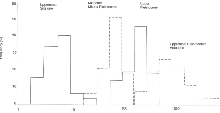
Worthington (1978) created a histogram of surface measured Formation resistivities and
20 divided the geological succession into four geo-electric units (Figure 3.1). Meyer et al.
(2001) extended the geological succession to five units. Table 3.1 is the extended biostratigraphic, Lithostratigraphic and geoelectric subdivision of the Cenozoic and Mesozoic succession as reported by Meyer et al. (2001). The list of the variation in the apparent resistivity of the geological Formation were obtained from borehole information and direct current sounding done on the outcrops of the various geological Formations (Worthington, 1978; Meyer et al., 2001).
.
Figure 3.1: Histogram of surface measured formation resistivities based on calibrations soundings (Worthington, 1978).
21 Table 3.1: Correlation of the biostratigraphic, Lithostratigraphic and geoelectrical subdivision of the Cenozoic and late Mesozoic succession on the Zululand Coastal Plain (Meyer et al., 2001).
Biostratigraphic
range Lithostratigraphic
range Geoelectric
range Resistivity range (ohm.m)
Approximate
position of geological Formations
Holocene- latest
Pleistocene Dune and beach
sand Surficial Unit
1(a) and 1 (b) 250 -7 500 Berea Formation Late Pleistocene Fine-grained
Aeolian quartz sand Upper Pleistocene unit 2
90 - 350 Bluff Formation
Middle
Pleistocene very fine- grained
quartz sand Middle Pleistocene
Unit 3(a) 24 -75 Port Durnford & Uloa Formations
Middle
Palaeocene Calcarenites,
coquina Miocene unit
3(b) Late Cretaceous Glauconite Palaeocene
Unit 4(a) 8 - 15 St Lucia Formation
Siltstone Late
Cretaceous Unit 4(b)
3 - 8 Mzinene Formation
Worthington (1978) analysed the aquifer pollution potential in the Mzingazi catchment and subdivided the area into 5 zones, and advised that there will be serious implications on the surface water regime of the Mzingazi catchment if the development of the residential areas is not controlled. These zones are also applicable in the areas around Richards Bay.
Meyer et al. (2001) concluded that at a regional scale, the undesirable land use practices are likely to affect the water resource in the area and recommended careful planning of new settlement and agricultural practice. The report further adds that seawater intrusion is not a major threat due to the elevated groundwater levels near the coast and the presence of the dunes acting as barriers. However on a large scale abstraction near the coastline might be something to look out for in case it reverses the flow direction of groundwater, therefore affecting the quality of water resources in the region.
Meyer et al. (2001) conducted 68 Transient Electromagnetic Soundings (TEM) in the Zululand coastal area. Some of the TEM were done at the same location as the direct current soundings in order to evaluate the TEM results.TEM method is very effective in
22 identifying conductive layers, whereas the direct current method identifies both conductive and resistive layers as long as they are well defined in terms of thicknesses, and that is why direct current in the Zululand coastal area is always preferred over TEM.
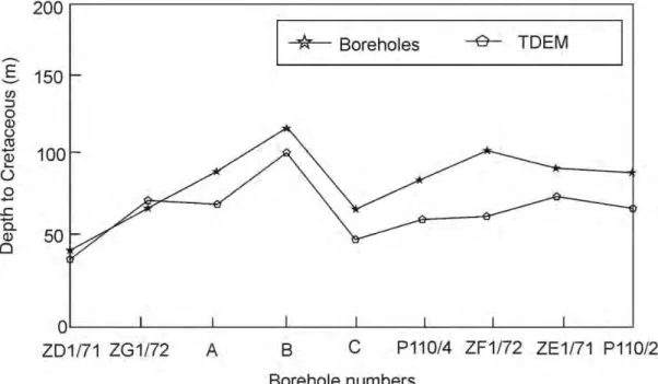
Only two cases recorded excellent correlation between what was recorded and the actual borehole results, the rest of the cases the Cretaceous floor was more than 20 m deeper than the interpreted depth to the conductive layer from the TEM results (Figure 3.2). The TEM reported by Meyer et al. (2001) defined the first conductive layer very well, but it’s not clear as to whether the layer represents the lower Port Durnford or the Cretaceous Formations. The electromagnetic sounding technique is not as extensively used as the direct current technique, mainly because of the expensive equipment and complicated interpretation methods (Fitterman and Stewart, 1986).
Figure 3.2: Comparison between the results of time domain electromagnetic sounding interpretations (TDEM) and drilling results (modified from Mayer et al., 2001).
23 3.3 Water balance
The water balance forms basis of analyzing the hydrology of a system, and used as a prediction tool for possible changes in a system. It also quantifies all the input and output parameter within a system by using directly measured and calculated parameters, such as precipitation, recharge, evaporation, evapotranspiration, runoff, base flow, the rate of abstraction and the change in storage.
3.3.1 Recharge estimation
Groundwater recharge can be defined as the downward movement of water that percolates the ground through the unsaturated zone reaching to the water table, hence adding to the groundwater reservoir (Sergio, 1997). Recharge is usually a small percentage of the annual precipitation over the area, but it’s highly important in the water balance estimation since it sustain the groundwater storage that has a direct effect on the streams, lakes and wetlands (Sergio, 1997). Groundwater is added into the aquifer in a number of methods such as gravitational flows from surface water sources such as lakes, rivers, rainfall, moist soil, wetlands and estuaries; lateral flows from adjoining aquifers and from dispersion within aquifers (Kelbe and Germishuyse, 2010). Bredenkamp et al. (1995) and Beekman and Xu (2003) have reviewed the methods of quantifying recharge to groundwater in the South African context. Van Tonder and Xu (2000) reviewed nine methods of estimating groundwater recharge, where they reported that no single method will produce good estimates of recharge in all cases. They developed recharge estimation methods using an Excel program called RECHARGE, which estimates effective recharge.
The methods included in the Excel RECHARGE program include the Chloride Mass Balance method (CMB), Isotope method, Water balance method, Cumulative Rainfall Departure (CRD) method, EARTH model, Carbon-14, Groundwater Model, Qualified guesses and spring flow analysis methods. The review further noted that in the cases where monthly abstraction rates and water levels in boreholes are known in an aquifer, a groundwater flow model, the SVF and CRD methods will usually be superior to other methods.
24 3.3.1.1 Chloride Mass Balance
This is by far the simplest tracer method for estimating groundwater recharge, and is the most inexpensive method. The method uses chloride (Cl-) as an environmental tracer, because of it conservative nature and its abundance in precipitation. The method has been applied in quite a number of investigations, to name a few, Eriksson and Khunakasem (1969); Sharma and Hughes (1985); Johnston (1987); Johansson (1987); Dettinger (1989): De Vries and Gieske (1990), Gieske (1992), Bazuhair and Wood (1996), Allison et al. (1994), Meinardi (1994) and the most recent and by far the most relevant in relation to the current research study is by Selaolo (1998).
The CMB method has been used to evaluate recharge processes in a wide range of environments, including the semi-arid environment with fractured rock aquifers (Cook et al., 2003), the saturated zones by Eriksson and Khunakasem (1969), in order to estimate recharge on the coastal plain of Israel, and in unsaturated zones as well, by comparing chloride concentrations in groundwater with the chloride deposition at the surface.
The method compares the total chloride deposition at the surface with the concentration in groundwater (Allison et al., 1984). The chloride concentration increases relative to the concentration of rainwater as a result of interception, soil evaporation and root water uptake by vegetation, in this light vegetation cover is vital in assessing the recharge potential at a site, because when vegetation at a specific area is high, the recharge of the groundwater tends to be low (Gee et al., 1994). The total chloride deposition and the total precipitation depth determine the chloride concentration of the rainwater at the surface (Allison et al., 1984). For diffusion conditions, the chloride increases in the root zone until a constant value below the constant zone is reached. Whereas under steady state conditions of piston flow, the flux of chloride at the surface is equal to the flux of chloride below the active root zone (Allison et al., 1984). The following are assumption made when applying the method (Allison et al., 1984):
The chloride ion behaves conservatively, i.e. it is not taken up by or leached from vegetation, unsaturated zone sediments or aquifer Formations.
25
Atmospheric input of chloride consisting of wet and dry depositions, is normally considered to be constant with time over longer periods, so long term and continuous monitoring is advisable in order to derive long term averages.
A piston flow regime is assumed, but can be invalidated by complex transport of moisture vertically and horizontally and this may occur in unsaturated zones as a result of the variability of in rainfall and evapotranspiration or uneven topography.
Preferential flow paths need to be attended to, as the soil moisture and solutes may be transported through the unsaturated zone by these pathways.
Recently the method has been used in a study done by Meyer et al. (2001) on the Zululand coastal plain and was a success. The recharge estimate ranged between 5-18 mm/year.
The CMB method is more effective when used in conjunction with other methods, since the chloride used may not be entirely from rain water, it may be from the weathering product of rocks, and therefore this method gives a minimum rate of recharge (Banks et
al., 2009).
3.3.2 Runoff Estimation
Runoff is important in determining catchment water balance. Runoff is defined as the amount of precipitation that runoff the surface (Tripathi and Singh 1998). The amount of runoff depends on precipitation, vegetation covering the land-surface, soil types and degree of disturbance, catchment slope and the water bodies in the catchment area. The Soil Conservation Service (SCS) in the early 1950’s conducted a study around small watershed in the United States to develop a method of estimating direct runoff from storm rainfall and the effect the land cover had on the volume of direct runoff.
The method was originally developed for small agricultural watersheds using daily rainfall data. The following are the limitations that are encountered in applying the method (USDA, 1986):
In the development of the equation, the time distribution and storm duration were not taken into consideration.
26
The equation tends to over predict runoff volume for discontinuous storm, because it does not account for the recovery of soil storage caused by infiltration during periods of no rain.
The CN procedure does not work well in areas where large proportion of flow is subsurface, rather than direct runoff.
Since the SCS curve numbers were developed from annual maximum one-day runoff data, the CN procedure is less accurate when dealing with shorter than one day runoff events.
The equation predicts that infiltration rate will approach zero for storms with long duration instead of a constant terminal infiltration rate.
The Rational method is another way of estimating runoff from rainfall, first developed by Mulvaney (1951) to solve problems related to land drainage. The method was later applied to sewer design in England and recently Tripathi and Singh (1998) conducted studies on small basins in India and developed the following relationship for estimating the peak discharge:
Q = 1/360 CIA (1)
Where C is the coefficient of runoff and is dependent on the catchment characteristics, I is the intensity of rainfall (mm/h); A is the area of the basin (ha) and Q is the peak rate of runoff in m3/s. C varies from 0.05 to 0.95 for flat sandy areas to impervious urban surfaces, respectively. Knowledge of the area is very important in the estimation as it helps the user to estimate the acceptable values (Shaw, 1994). Value also varies for different storms of the same catchment, therefore using the average value gives crude runoff estimate which may have a wide margins of error. Weitz and Demlie (2014) used the rationale method on the Sibayi catchment adjacent to the Kosi Bay catchment to estimate runoff rate from the catchment to the lake.
3.3.3 Evapotranspiration
Evapotranspiration represents two terms describing separate processes that occur hand in hand through the natural system. During the process water is lost from the soil by
27 evaporation and from the actual vegetation through transpiration at the same time.
Evapotranspiration can be estimated as reference crop evapotranspiration (Allen et al., 1998). Empirical formulas of international standards such as the Bleney-Criddle, radiation, modified Penman-Monteith and pan evaporation methods are used to estimate the crop evapotranspiration. The Bleney-Criddle method is essentially for areas that have air temperature data only, which makes the estimated value less accurate. The method is also recommended for periods of one month or more. The Radiation method is for areas with measured air temperature and sunshine duration, radiation, wind speed and relative humidity data. The method is recommended for ten day or monthly evapotranspiration calculation. Pan evaporation method can be used for periods of ten days or even longer.
The FAO Penman-Monteith method also needs climatic data such as air temperature, relative humidity, radiation and wind speed data for daily, weekly, ten-day or monthly calculations (Allen et al., 1998).
In the analysis of the accuracy and performance of the above evapotranspiration estimation methods, studies were undertaken by Committee on Irrigation Water Requirements of the American Society of Civil Engineers (ASCE) in 11 locations with variable climatic conditions and in the European Community by a consortium of European research institutes. The studies showed that different methods performed differently from place to place. The following are observation from the analysis in each of the methods implemented (Allen et al., 1998):
The Penman methods may require local calibration of the wind function to achieve satisfactory results.
The radiation methods show good results in humid climates where the aerodynamic term is relatively small, but performance in arid conditions are erratic and tend to underestimate evapotranspiration.
Temperature methods remain empirical and require local calibration in order to achieve satisfactory results. A possible exception is the 1985 Hargreaves’
method that has shown reasonable ETo results with a global validity.
Pan Evapotranspiration methods clearly reflect the shortcomings of predicting crop evapotranspiration from open water evaporation. The methods are
28 susceptible to the microclimatic conditions under which the pans are operating and the consistency of station maintenance. Their performance proves erratic.
The relatively accurate and consistent performance of the Penman-Monteith approach in both arid and humid climates has been indicated in both the ASCE and European studies.
Allen et al. (1998) developed the FAO Penman-Monteith method to estimate reference crop evaporation. This is a combination of the aerodynamic equation and the resistance equation. In practice, the reference evapotranspiration is different from the crop evapotranspiration (ETc) because the different areas in the field are not necessarily covered by grass. So in order to account for this, the crop coefficient (Kc) was introduced to account for the physiological and physical difference in crops. Therefore, the crop evapotranspiration is the product of ETo and Kc (Allen et al., 1998).
3.3.4 Open Water Evaporation
Evaporation is one of the most difficult components of the hydrological cycle to quantify, but is very important as it accounts for the large differences that occur between incoming precipitation and water available in the open water bodies. Evaporation can be defined as the transfer of water from open water sources such as the lakes, rivers, streams and reservoirs to the atmosphere, and is influenced by the general climate of the area. There are quite a few techniques to quantify evaporation, directly and indirectly. The direct methods include the use of instruments such as evapotron (Dyer and Maher, 1965). The indirect methods include the water budget method. Tanks and pans are some of the instruments that can be used in quantifying evaporation even though they may prove to be more difficult when it comes to relating measurements from small bodies to the real losses from a large reservoir.
In this research, the Penman (1948) Formula is used to calculate the open water evaporation. This Formula has been used all over the world, especially by practicing engineers. The formula is based on the fundamental physical principles with some empirical concept, and uses meteorological data, combining both the mass transfer method and the energy budget method. The mass transfer method calculates the upward flux of water vapour from the evaporation surface. The energy budget method considers
29 the heat sources and sinks of the water body and air and isolates the energy required for the evaporating process (Shaw, 1994).
3.4 Analysis and modelling of groundwater-surface water interactions Historically, groundwater and surface water have been discussed in literature as separate entities because of their general different properties. However, in actual fact understanding the processes that develop as a result of surface water-groundwater interactions are becoming more important to protect the integrity of related surface water ecosystems, such as rivers, lakes and wetlands (Kelbe and Germishuyse, 2010). The declaration of the National Water Act (Act 36 of 1998) and the recognition of the connection and the interdependence of groundwater and surface water in the hydrological cycle has required a more holistic approach. As a result of closer working relationships, it has shown that the understanding of surface water - groundwater interaction is poor and many previous hydrological investigations have not addressed this issue adequately and failure to address the issue might perpetuate the poor decision making in the assessment and management of the precious water resources (Kelbe and Germishuyse, 2010).
A simple conceptual models can be very useful in evaluating the groundwater interaction with the surface water bodies, and there are several methods that can be used to achieve it. The conceptual model should consider the main features of the aquifer and the response in the surface water bodies.
Considering the assumption of mass balance approach, any change in surface water (loss or gain) can be related to groundwater. Therefore the change can be identified and measured. The interaction of groundwater and surface water can be determined using a number of methods depending on the type of environment and water body under consideration.
Conceptual and numerical models are useful tools to improve our current understanding of surface water- groundwater interaction. As much as modelling may be a useful tool, failure to calibrate models using measured data merely perpetuates our flawed conceptual