The invasive potential of the freshwater snail Radix rubiginosa recently introduced into South Africa.

(1)

________________________________________________________________________

The invasive potential of the freshwater snail Radix rubiginosa recently introduced into South Africa

________________________________________________________________________

By

Devandren Subramoney Nadasan

Submitted in fulfillment of the academic Requirements for the

Degree of Doctor of Philosophy in the

School of Biological and Conservation Sciences University of KwaZulu-Natal,

Westville Campus Durban, South Africa 2011

As the candidate’s supervisor I have approved this dissertation for submission.

____________________________ __________________

Professor C.C. Appleton Date

(2)

________________________________________________________________________

Dedication

________________________________________________________________________

This dissertation is dedicated to my parents. I love you Mum and Dad, for helping to make me who I am, for teaching me to be proud of who I am, for showing me how to be strong, for giving me the courage and strength to always strive for better, no matter what. Thank you for giving me the wisdom to know when to turn away and when to charge ahead...you are my rock and foundation.

(3)

________________________________________________________________________

Abstract

________________________________________________________________________

Invasions of ecosystems by exotic species are increasing and they may often act as a significant driver of the homogenization of the Earth’s biota, resulting in global

biodiversity loss. Moreover, the addition of exotic species may have dramatic effects on ecosystem structure and functioning which may result in the extirpation of indigenous species. In 2004, a large population of an unknown lymnaeid was found in the

Amatikulu Hatchery, northern KwaZulu-Natal, South Africa, and was subsequently found in few garden fish ponds in Durban. In 2007, it was identified using molecular techniques as Radix rubiginosa (Michelin, 1831) – a species widespread in southeast Asia. An invasion by R. rubiginosa is however likely to go unnoticed because its shell morphology resembles some forms of the highly variable and widely distributed indigenous lymnaeid, Lymnaea natalensis Krauss, 1848.

Accurate and “easy” species identifications would permit the ready assessment of

introduction histories and distributions, but in the present case identification was difficult due to unclear and contradicting accounts of the indigenous L. natalensis in the literature.

A redescription of L. natalensis with emphasis on conchological and anatomical

characteristics was therefore presented. This will help to distinguish variation between R.

rubiginosa and L. natalensis and also assist those carrying out rapid bioassessment (SASS) surveys in South African rivers in recognising R. rubiginosa should it spread.

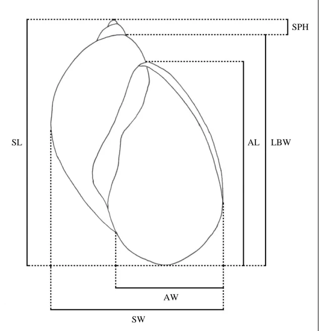
For this, shells of R. rubiginosa and L. natalensis from both the UKZN Pond and the Greyville Pond were selected into either size class 1 (shell length < 10 mm) or size class 2 (shell length ≥ 10 mm). Six shell characters, shell length (height), shell width, aperture length (height), aperture width, length of last body whorl and spire height for each specimen was measured and analysed using principal component analysis (PCA) and

(4)

discriminant functions analysis (DFA). The most useful discriminant conchological characters were shell length, length of the last body whorl and aperture width. Use of these shell characters provided simple yet effective criteria for the separation of R.

rubiginosa and L. natalensis. For both size classes R. rubiginosa had larger, more broadly ovate shells with longer (higher) body whorls than either of the two populations of L. natalensis that exhibited smaller, elongated shells with shorter (lower) body whorls.

Also, R. rubiginosa had a narrower aperture width compared to the larger, wider aperture of the UKZN Pond L. natalensis population. The Greyville L. natalensis population was found to have narrower apertures than both R. rubiginosa and L. natalensis (UKZN Pond).

The morphology of the radula and the reproductive anatomy of R. rubiginosa and L.

natalensis from both the UKZN and Greyville Ponds showed little variation. The species did however vary in the relative numbers of radula teeth in each field and this serves as an additional useful diagnostic character. Both L. natalensis populations had similar mantle pigmentation patterns but that of R. rubiginosa was different. The mantle surface of R. rubiginosa was mottled black with patches of pale white to yellow. There were also large unpigmented fields and stripes that were not observed in L. natalensis. Having found characters to conveniently separate the alien R. rubiginosa from the indigenous L.

natalensis, it became increasingly important to assess the potential invasiveness of this introduced species and its likely impact.

The potential invasiveness of R. rubiginosa was assessed in relation to the already invasive North American Physidae Physa acuta Draparnaud, 1805 and the indigenous L.

natalensis. This was particularly important in view of the success of P. acuta as an invader in South Africa. The hatching success, frequency of egg abnormalities, embryonic development, growth, survivorship, fecundity and life history parameters (GRR, Ro, rm, T and λ) for the four snail populations were assessed at three experimental temperatures (20ôC, 25ôC and 30ôC).

(5)

The results showed that R. rubiginosa and P. acuta had a higher growth coefficient (K), longer survivorship, higher fecundity (higher hatching success, fewer egg abnormalities, longer duration of oviposition), shorter incubation period, greater life history parameters (GRR, R_o, r_m and λ) and wider temperature tolerances than the two L. natalensis

populations tested.

The high adaptability of P. acuta to changing environmental factors such as temperature, is in agreement with the fact that it is now more widespread in South Africa than the indigenous species L. natalensis. This has important implications for R. rubiginosa, since this species displayed reproductive attributes and a temperature tolerance that were similar and in certain cases even exceeded the performance of the invasive P. acuta. This therefore implies that R. rubiginosa has the potential to colonize a wider geographical and altitudinal range than L. natalensis, and perhaps even P. acuta. Also, the superior reproductive ability of R. rubiginosa over L. natalensis is likely to present a situation that allows for its rapid spread as well as a possible impact on the indigenous L. natalensis that might render it vulnerable.

(6)

________________________________________________________________________

Preface

________________________________________________________________________

The research work described in this dissertation was carried out in the School of

Biological and Conservation Sciences, University of KwaZulu-Natal, Westville Campus, Durban under the supervision of Professor C.C. Appleton.

These studies represent original work by the author and have not otherwise been submitted in any form for any degree or diploma to any tertiary institution. Where use has been made of the work of others, it is duly acknowledged in the text.

____________________________

Devandren Subramoney Nadasan

(7)

________________________________________________________________________

Acknowledgements

________________________________________________________________________

This endeavour to complete my doctoral degree and dissertation could never have been accomplished without the support and assistance of so many over the years.

I would want to express my heart-felt gratitude to God Almighty, whose blessings have accompanied me every step of my academic pursuits.

A special thanks to my supervisor, Professor C.C. Appleton, whose wisdom and

knowledge has guided this research from its inception. His support, guidance and advice throughout this study, as well as his painstaking effort in critically reviewing the drafts are greatly appreciated. I am also grateful for the confidence he showed in both me and my research, and for his constructive supervision and stimulating discussion. Thank you for being an enthusiastic collaborator and tutor and sharing your broad knowledge selflessly with me.

I wish to express my sincere gratitude and appreciation to the following individuals who assisted in various aspects of this study:

I am grateful to staff members of the School of Biological and Conservation Sciences, Westville Campus for the provision of facilities and equipment used for the duration of the study.

The staff of the Electron Microscope Unit (University of KwaZulu-Natal, Westville Campus) for their invaluable assistance, support and advice with the microscopy studies.

(8)

I would also want to thank my friends and fellow colleagues for their academic

inspiration, and for sharing experiences and friendship throughout a long and not always easy road with me.

A special thanks to my loving wife, Terusha for her support and encouragement. Thank you for playing an important role along my journey, as we mutually engaged in making sense of the various challenges we faced and in providing continuous encouragement, understanding and inspiration.

Funding for the duration of the study was provided through Prestigious and Equity Scholarships awarded by the National Research Foundation (NRF) of South Africa. In addition, financial assistance from the University of KwaZulu-Natal, Westville Campus is duly acknowledged.

My heart-felt thanks to my parents and brothers for the myriad ways in which they have supported me in my determination to find and realise my potential. Thank you for the unconditional love, prayer, encouragement and support. I love you all.

(9)

________________________________________________________________________

List of Contents

________________________________________________________________________

Dedication...

Abstract...

Preface...

Acknowledgements...

List of Contents...

List of Tables...

List of Figures...

ii iii vi vii ix xvi xxii

Chapter 1 General Introduction

1.1 Biological Invasions...

1.2 Factors affecting Biological Invasions...

1.3 Impacts of Biological Invasions...

1.4 Invasive freshwater snails in South Africa...

1.5 First Report of Radix rubiginosa in South Africa...

1 2 3 4 4

Chapter 2

Review of the Family Lymnaeidae

2.1 The systematic – taxonomic confusion in the family Lymnaeidae...

2.2 Phylogeny of the Family Lymnaeidae...

2.2.1 Shell Characters and their use in Phylogeny...

2.2.2 Anatomical Characters and their use in Phylogeny...

2.2.3 Biochemical and Molecular Studies and their use in Phylogeny...

8 9 9 10 11

(10)

2.3 Lymnaeids in parasite transmission...

2.4 Conservation status of the Lymnaeidae...

12 14

Chapter 3

Redescription of Lymnaea natalensis Krauss, 1848 from its type locality

3.1 Introduction...

3.2 Methodology...

3.2.1 The Study Site...

3.2.2 Shell Morphology...

3.2.3 Anatomical Morphology...

3.2.3.1 Radula...

3.2.3.2 Mantle pigmentation patterns...

3.2.3.3 Reproductive Anatomy...

3.3 Classification and Distribution of Lymnaea in Africa...

3.4 Results...

3.4.1 Original Description...

3.4.2 Shell Morphology...

3.4.3.1 Radula...

3.5 Discussion...

3.6 Appendix to Chapter 3...

16 18 18 20 21 21 22 22 23 27 27 28 29 29 33 34 38 42

(11)

Chapter 4

Morphological and Anatomical Variation in Radix rubiginosa and Lymnaea natalensis

4.1 Introduction...

4.2 Methodology...

4.2.1 The Malacological Study Sites...

4.2.1.1 Amatikulu Prawn and Fish Hatchery (Amatikulu)...

4.2.1.2 UKZN Pond (Cato Manor, Durban)...

4.2.1.3 Greyville Race Course (Greyville, Durban)...

4.2.2 Snail species occurring in the study areas...

4.2.3 Vegetation types present in the study areas...

4.2.4 Shell Morphology and Morphometrics...

4.2.4.1 Characters selected for Shell Morphometric Analysis...

4.2.4.2 Statistical Morphometric Analyses...

(a) Error Measurements...

(b) Principal Component Analysis (PCA)...

(c) Discriminant Functions Analysis (DFA)...

4.2.5.1 Radula...

4.3 Results...

4.3.1.1 Shell Description...

(a) Radix rubiginosa (Amatikulu Prawn and Fish Hatchery)...

(b) Lymnaea natalensis (UKZN Pond)...

(c) Lymnaea natalensis (Greyville Pond)...

4.3.1.2 Error Measurements...

4.3.1.3 Normality, Skewness and Kurtosis...

4.3.1.4 Size Class 1 (shell length < 10mm)...

45 49 49 50 52 52 53 55 55 55 57 57 59 59 60 60 60 60 61 61 61 61 62 63 64 65 67

(12)

(a) Principal Component Analysis...

(b) Discriminant Function Analysis...

4.3.1.5 Size Class 2 (shell length ≥ 10mm)...

(a) Principal Component Analysis...

(b) Discriminant Function Analysis...

4.3.2.1 Radix rubiginosa...

(a) Radula...

(b) Mantle pigmentation...

(c) Reproductive Anatomy...

4.3.2.2 Lymnaea natalensis (UKZN Pond)...

(a) Radula...

(b) Mantle Pigmentation...

4.3.2.3 Lymnaea natalensis (Greyville Pond)...

(a) Radula...

(b) Mantle Pigmentation...

4.4 Discussion...

67 68 70 70 71 74 74 74 78 79 80 80 80 80 81 81 84 85 86 87 89

Chapter 5

Embryonic Development of Radix rubiginosa, Lymnaea natalensis and Physa acuta

5.1 Introduction...

5.2 Methodology...

5.2.1 Egg Abnormalities, Viable Eggs and Hatching Success...

5.2.1.1 Egg Abnormalities...

5.2.1.2 Viable Eggs and Egg Hatching Success...

5.2.2 Embryonic Development...

91 94 94 94 95 95

(13)

5.3 Results...

5.3.1 Description of Egg Capsules...

(a) Radix rubiginosa...

(b) Lymnaea natalensis...

(c) Physa acuta...

5.3.2 Viability of Eggs and Egg Abnormalities...

(a) Hatching Success...

(b) Dwarf Eggs...

(c) Eggs without Egg Cells...

(d) Eggs without Development...

(e) Polyvitelline Eggs...

5.3.3 Embryonic Development...

(a) Egg Cell before Cleavage...

(b) First Cleavage (2-cell stage)...

(c) Second Cleavage (4-cell stage)...

(d) Third Cleavage (8-cell stage)...

(e) Fourth Cleavage (16-cell stage)...

(f) Fifth Cleavage (24-cell stage)...

(g) Sixth Cleavage (64-cell stage)...

(h) Blastula Stage...

(i) Gastrula Stage...

(j) Early Trochophore Stage...

(k) Late Trochophore Stage...

(l) Early Veliger Stage...

(m) Late Veliger Stage...

(n) Hatching Stage...

5.3.3.1 Analysis of the incubation period, mean size and mean geometric growth rate...

5.4 Discussion...

5.4.1 Egg Capsule Descriptions...

5.4.2 Viability of Eggs and Egg Abnormalities...

97 97 99 100 100 101 101 102 103 103 103 108 108 108 110 111 113 114 114 115 115 117 118 119 120 121 122 128 128 129

(14)

(a) Hatching Success...

(b) Dwarf Eggs...

(c) Eggs without Egg Cells...

(d) Eggs Without Development...

(e) Polyvitelline Eggs...

5.4.3 Embryological Development...

129 129 130 131 131 133

Chapter 6

Growth and Life History Parameters of Radix rubiginosa, Lymnaea natalensis and Physa acuta

6.1 Introduction...

6.2 Methodology...

6.2.1 Growth...

6.2.2 Survival, Fecundity and Life History Parameters...

(a) Age (x)...

(b) Survival rate (lx)...

(c) Fecundity (mx)...

(d) Gross reproductive rate (GRR)...

(e) The net reproductive rate (Ro)...

(f) Intrinsic rate of natural increase (rm)...

(g) Mean generation time (T)...

(h) Finite rate of increase (λ)...

6.3 Results...

6.3.1 Growth...

6.3.2 Survival Rate...

6.3.3 Fecundity...

6.3.4 Life History Parameters...

(a) Gross Reproductive Rate (GRR)...

(b) The net reproductive rate (Ro)...

(c) Intrinsic rate of natural increase (rm)...

136 139 139 140 141 141 141 142 142 142 143 143 144 144 151 157 164 164 169 170

(15)

(d) Mean generation time (T)...

(e) Finite rate of increase (λ)...

6.4 Discussion...

6.4.1 Growth...

6.4.2 Survival Rate...

6.4.3 Fecundity...

6.4.4 Life History Parameters...

(a) Gross Reproductive Rate (GRR)...

(b) The net reproductive rate (R_o)...

(c) Intrinsic rate of natural increase (r_m)...

(d) Mean generation time (T)...

(e) Finite rate of increase (λ)...

171 171 173 174 176 177 179 179 180 180 182 183

Chapter 7

General Discussion and Conclusions...

References...

186 200

(16)

________________________________________________________________________

List of Tables

________________________________________________________________________

Chapter 3

Table 3.1: Selected water chemistry parameters for the UKZN Pond. All values

measured are indicated as mean (± standard deviation), n = 35... 19

Chapter 4

Morphological and Anatomical Variation in Radix rubiginosa and Lymnaea natalensis

Table 4.1: Selected water chemistry parameters for the three study sites. All values measured are indicated as mean (± standard deviation), n = 35...

Table 4.2: Snail species identified from the three study sites. (+) indicates

presence; (-) indicates absence...

Table 4.3: Aquatic plant species present in the three study sites. (+) indicates presence; (-) indicates absence...

Table 4.4: Descriptive statistics for the six shell characters (n = 30), arranged in order of increasing percentage measurement error (%ME). CVWI = overall within- individual error and CVBI = overall between-individual error. Minimum (min), maximum (max) and mean values are provided for each character. To assess the associated error levels, 30 individuals with a complete suite of shell characters were randomly chosen, five individuals from each of the three study sites and the

52

54

55

(17)

two size classes………....

Table 4.5: Basic statistics (arithmetic mean and standard deviation) for the six shell characters of size class 1 (shell length < 10 mm) from the three study sites (n

= 100). The results of the normality (Kolmogorov-Smirnov Test), skewness (g₁) and kurtosis (g2) tests are also given...

Table 4.6: Basic statistics (arithmetic mean and standard deviation) for the six shell characters of size class 2 (shell length ≥ 10 mm) from the three study sites (n

= 100). The results of the normality (Kolmogorov-Smirnov Test), skewness (g₁) and kurtosis (g₂) tests are also given...

Table 4.7: Component loadings (correlation coefficients) of shell morphological characters for R. rubiginosa and L. natalensis from size class 1 (shell length < 10 mm). The component loadings were derived from principal component analysis of the six shell characters after natural logarithm transformation. Values with the highest component loadings are in bold...

Table 4.8: Standardised canonical discriminant function coefficients of principal component loadings for R. rubiginosa and L. natalensis from size class 1 (shell length < 10 mm). Only the results of those parameters that contributed

significantly to the DFA model are shown...

Table 4.9: Component loadings (correlation coefficients) of shell morphological characters for R. rubiginosa and L. natalensis from size class 2 (shell length ≥ 10 mm). The component loadings were derived from principal component analysis of the six shell characters after natural logarithm transformation. Values with the highest component loadings are in bold...

64

66

67

68

70

(18)

Table 4.10: Standardised canonical discriminant function coefficients of principal component loadings for R. rubiginosa and L. natalensis from size class 2 (shell length ≥ 10 mm). Only the results of those parameters that contributed

significantly to the DFA model are shown... 71

Chapter 5

Table 5.1: Comparison of egg capsule dimensions and clutch sizes for each of the four snail populations (n = 100). Dimensions are presented as mean millimeters (±

standard error)...

Table 5.2: Hatching success and egg abnormalities (%) for the four snail populations at the three temperatures (n = 25). The values are presented as

percentage means (± standard deviation)...

Table 5.3: Kruskal-Wallis analysis of the influence of temperature on viable eggs (hatching success) and egg abnormalities for the four snail populations (n = 25).

Probability values are two-tailed and significance was determined at p < 0.05...

Table 5.4: Kruskal-Wallis analysis for viable eggs (hatching success) and egg abnormalities between snail populations maintained at 20^oC (n = 25). Probability values are two-tailed and significance was determined at p < 0.05...

Table 5.5: Kruskal-Wallis analysis for viable eggs (hatching success) and egg abnormalities between snail populations maintained at 25^oC (n = 25). Probability values are two-tailed and significance was determined at p < 0.05...

Table 5.6: Kruskal-Wallis analysis for viable eggs (hatching success) and egg abnormalities observed between snail populations maintained at 30^oC (n = 25).

99

102

104

105

106

107

(19)

Table 5.7: Incubation period, mean size and mean geometric growth rate (GGR) of the different embryonic stages of development for R. rubiginosa at the three

temperature treatments (n = 15). Mean sizes of embryo are given in millimetres (±

standard deviation). Gaps in the incubation periods between embryonic stages are due to an absence of synchronous development...

Table 5.8: Incubation period, mean size and mean geometric growth rate (GGR) of the different embryonic stages of development for L. natalensis (UKZN pond) at the three temperature treatments (n = 15). Mean sizes of embryo are given in millimetres (± standard deviation). Gaps in the incubation periods between

embryonic stages are due to an absence of synchronous development...

Table 5.9: Incubation period, mean size and mean geometric growth rate (GGR) of the different embryonic stages of development for L. natalensis (Greyville pond) at the three temperature treatments (n = 15). Mean sizes of embryo are given in millimetres (± standard deviation). Gaps in the incubation periods between

embryonic stages are due to an absence of synchronous development...

Table 5.10: Incubation period, mean size and mean geometric growth rate (GGR) of the different embryonic stages of development for P. acuta at the three

temperature treatments (n = 15). Mean sizes of embryo are given in millimetres (±

standard deviation). Gaps in the incubation periods between embryonic stages are due to an absence of synchronous development...

Table 5.11: Kruskal-Wallis analysis for the size of the embryonic stages of development for the four snail populations as a function of temperature (n = 15).

123

124

125

126

127

(20)

Chapter 6

Table 6.1: Estimated growth parameters of the four snail populations maintained at the three temperatures. These parameters were estimated using the Ford-Walford method...

Table 6.2: Analysis of the mean age specific survival rate (l_x) within the four snail populations, for each of the three temperatures (n = 90). Differences in survival rates within populations were analysed using the Mann-Whitney-U test.

Table 6.3: Analysis of the mean age specific survival rate (lx) for the four snail populations, maintained at the three temperatures (n = 90). Differences in survival rates between populations were analysed using the Mann-Whitney-U test.

Table 6.4: Analysis of the mean age specific fecundity (mx) for the four snail populations at each of the three temperatures (n = 3). Differences in fecundity within populations and between temperatures were analysed using the Mann- Whitney-U test. Probability values are two-tailed and significance was determined at p < 0.05...

Table 6.5: Analysis of the mean age specific fecundity (mx) for the four snail populations maintained at the three temperatures (n = 3). Differences in fecundity between populations were analysed using the Mann-Whitney-U test. Probability values are two-tailed and significance was determined at p < 0.05...

147

151

153

157

160

(21)

Table 6.6: Life history parameters of the four snail populations maintained at the three temperature treatments (n = 3). The values are based on a time interval of one week and are presented as means (± standard deviation)...

Table 6.7: Multiple comparisons using Tukey HSD. Life history parameters within the four snail populations were analysed for differences at each of the three temperatures (n = 3). Probability values are two-tailed and significance was

determined at p < 0.05...

Table 6.8: Multiple comparisons using Tukey HSD. Life history parameters between the four snail populations were analysed for differences at 20^oC (n = 3).

Table 6.11: Summary of the results for the age specific growth, survival, fecundity and life history parameters for each of the four snail populations………...

165

166

167

168

169

173

Chapter 7

General Discussion and Conclusions

Table 7.1: Examples of research on hypotheses of species invasiveness and

ecosystem invasibility... 188

(22)

________________________________________________________________________

List of Figures

________________________________________________________________________

Chapter 3

Figure 3.1: Map of KwaZulu-Natal showing the UKZN Pond study site (U), selected for the redescription of L. natalensis...

Figure 3.2: The UKZN Pond...

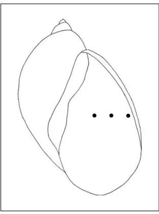
Figure 3.3: Schematic drawing of the shell indicating the points (●) where shell thickness was measured. The mean shell thickness was presented as μm (±

standard deviation)...

Figure 3.4: Lymnaea natalensis from Arabia, with the locality given in parentheses, scale bar 10 mm.

A-B, Lymnaea caillaudi (Mesajia, Yemen); C, Lymnaea muscatensis (Muscat); D- E, Lymnaea caillaudi (Kalhat, Saudi Arabia)...

Figure 3.5: Lymnaea natalensis from Madagascar, with the locality given in parentheses, scale bar 10 mm.

A-C, Lymnaea natalensis (Antisirabe, Madagascar); D-F, Lymnaea natalensis (Lake Renobe, Madagascar); G-H, Lymnaea pacifica (Ambatondigen,

Madagascar); I-J, Lymnaea specularis (Ankazoaba, Western Madagascar); K-O, Lymnaea hovarum (Antanamena, Madagascar); P, Lymnaea pacifica (Ankazoaba, Western Madagascar); Q, Lymnaea electa (Ankazoaba, Western Madagascar)...

18 20

21

23

24

(23)

Figure 3.6: Lymnaea natalensis from Africa, with the locality in which they were described given in parentheses, scale bar 10 mm.

A-B, Lymnaea exsertus (Sweet water Canal, Suez); C, Lymnaea pharaonum (Egypt); D, Lymnaea caillaudi (Alexandria, Egypt), E-G, Lymnaea caillaudi (Nuruya, Darfur); H-I, Lymnaea ribeirensis (San Antao Island, Cape Verde Island);

J-M, Lymnaea nyansae (Entebbe, Uganda); N, Lymnaea elmeteitensis (Northern Uganda); O-P, Lymnaea undussumae (Ndola Swamp, Northern Zimbabwe); Q, Lymnaea nyansae (Luanshyla, Northern Zimbabwe); R-S, Lymnaea caillaudi (Northern Zimbabwe); T-W, Lymnaea natalensis (Port Natal, South Africa); X-Y, Lymnaea natalensis (Durban, South Africa)...

Figure 3.7: The distribution of Lymnaea spp. in Africa and Madagascar.

Occurrences in the Cape Verde Islands are not shown on the map. According to Hubendick (1951) and later Brown (1994) there is little justification for

maintaining most of the many named species in Africa; the whole range seems to be inhabited by a single but variable species, Lymnaea natalensis. The shaded regions are intended to represent the main areas of occurrence, however, continuity of distribution is not implied and there may be significant discontinuities within the shaded areas...

Figure 3.8: The original description, in Latin and German, of L. natalensis transcribed from Krauss (1848: 85), supplemented with the original figure of the shell of a specimen from a lentic pool in what is now the city of Durban (see, Figure 15 in text)...

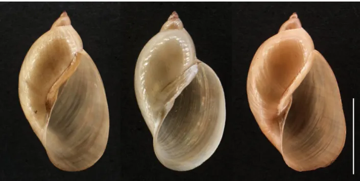
Figure 3.9: Shells of L. natalensis (UKZN Pond) showing the variation found in the population, scale bar 10 mm...

Figure 3.10: Scanning electron micrograph of the central tooth and lateral teeth of L. natalensis (UKZN Pond). A smaller accessory cusp is located on the central tooth (indicated by the arrow), scale bar 10 μm.

24

25

27

28

(24)

C – central tooth; L – lateral tooth...

Figure 3.11: Scanning electron micrograph of the lateral teeth from the left side of a transverse row of L. natalensis (UKZN Pond). For lateral teeth 6-8, the endocone and mesocone appeared very acute in shape and gradually became sub-equal in length, scale bar 10 μm...

Figure 3.12: Scanning electron micrograph of the intermediate laterals (9^th and 10^th pair of teeth) of L. natalensis (UKZN Pond). In the 9^th pair, the ectocone split into two smaller, acute-shaped denticles (indicated by the arrows). The ectocones of the 10^th pair did not split into two smaller denticles and they resembled the tricuspid shape and pattern of the 7^th and 8^th laterals, scale bar 10 μm.

IL – intermediate lateral tooth; L – lateral tooth; M – marginal tooth...

Figure 3.13: Scanning electron micrograph of the marginal teeth (indicated by numbers 3-12) of L. natalensis (UKZN Pond). The marginal teeth were multicuspid having four cusps that were short, bluntly rounded and obliquely placed, scale bar 10 μm...

Figure 3.14: Lymnaea natalensis (UKZN Pond) – animal with shell removed to show pigmentation patterns.

A – Dorsal view of animal showing the mantle pigmentation pattern, scale bar 10 mm.

B – Ventral view showing foot and mouth, scale bar 10 mm.

f – foot; m – mouth; vc – visceral coil; vm – visceral mass...

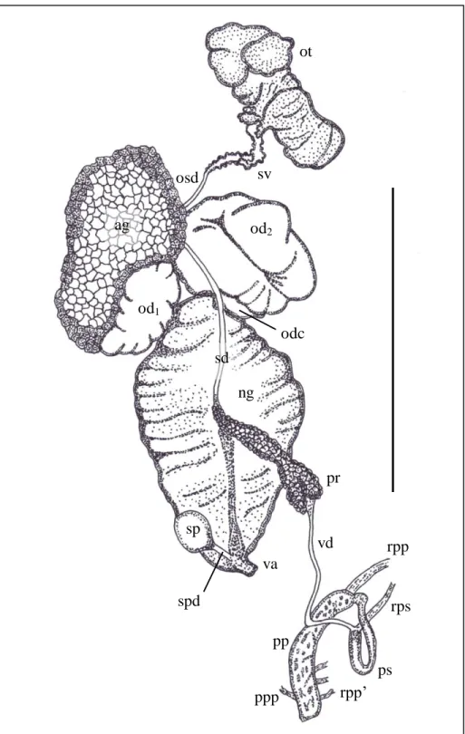
Figure 3.15: Reproductive anatomy of L. natalensis (UKZN Pond), scale bar 10 mm.

ag – albumen gland; ng – nidamental gland; od1 – proximal portion of oviduct;

od2 – distal portion of oviduct; odc – oviducal caecum; osd – ovispermiduct;

ot – ovotestis; pp – praeputium; ppp – protractor muscle of praeputium;

29

30

31

32

33

(25)

pr – prostate; ps – penial sheath; rpp – retractor muscle of praeputium;

rpp’ – smaller retractor muscle of praeputium; rps – retractor muscle of penial sheath; sd – spermiduct; sp – spermatheca; spd – spermathecal duct; sv – seminal vesicle; va – vagina; vd – vas deferens...

Figure A1.1: Tree based on 389 nucleotides of the 18SrRNA gene from lymnaeid samples, with the outgroup Stagnicola palustris. Tree constructed using

neighbour-joining method. Bayesian posterior probabilities, neighbour-joining and maximum parsimony bootstrap values were all very weak (<50%) and were thus omitted. The maximum parsimony tree obtained represented a strict consensus of 526 shortest trees. The scale of the branch length of 0.005 represents the number of substitutions per site.

LNA - samples from the Amatikulu Hatchery, Amatikulu, South Africa; LNP - samples from the Nwanetsi River in Mamitwa, Limpopo province, South Africa;

LNU - samples from the UKZN Pond, Durban, South Africa; LSV - samples from Hanoi, Vietnam...

Figure A1.2: Tree based on 533 nucleotides of the cytochrome oxidase subunit I gene of lymnaeid samples, with the outgroup Planorbis corneus. Tree constructed using neighbour-joining method. Numbers on branches represent Bayesian

posterior probabilities percentages, neighbour-joining and maximum parsimony bootstrap values, respectively. Only values greater than 50% are shown (*

indicates support of < 50% for distance analysis). The maximum parsimony tree obtained represented a strict consensus of 219 shortest trees. The scale of the branch length of 0.002 represents the number of substitutions per site.

LNA - samples from the Amatikulu Hatchery, Amatikulu, South Africa; LNU - samples from the UKZN Pond, Durban, South Africa.; LSV - samples from Hanoi, Vietnam...

Figure A1.3: Tree based on 360 nucleotides of the 16SrRNA gene of lymnaeid samples, with the outgroup Stagnicola elodes. Tree constructed using neighbour-

37

42

43

(26)

joining methods. Numbers on branches represent Bayesian posterior probabilities percentages, neighbour-joining and maximum parsimony bootstrap values

respectively. Only values greater than 50% are shown (* indicates support of

<50% for distance analysis). The maximum parsimony tree obtained represented a strict consensus of 210 shortest trees. The scale of the branch length of 0.002 represents the number of substitutions per site.

LNA - samples from the Amatikulu Hatchery, Amatikulu, South Africa; LNU - samples from the UKZN Pond, Durban, South Africa; LSV - samples from Hanoi, Vietnam... 44

Chapter 4

Morphological and Anatomical Variation in Radix rubiginosa and Lymnaea natalensis

Figure 4.1: Map of KwaZulu-Natal showing the study sites selected for sampling:

(1) – Amatikulu Prawn and Fish Hatchery (Amatikulu); (2) – UKZN Pond (Cato Manor, Durban); (3) – Greyville Race Course Pond (Greyville, Durban)...

Figure 4.2 A, B: The Amatikulu Prawn and Fish Hatchery (Amatikulu).

A - Aerial view of Hatchery (Courtesy of G. Upfold).

B - Inside view of tanks in a typical polytunnel...

Figure 4.3: The Greyville Pond...

Figure 4.4: Representatives of the family Lymnaeidae, identified from the study areas.

A – Lymnaea natalensis Krauss, 1848, scale bar 10 mm

B – Radix rubiginosa (Michelin, 1831), scale bar 10 mm...

Figure 4.5: Schematic drawing of the six shell characters used for the traditional morphometric approach.

AL – aperture length; AW – aperture width; LBW – length of last body whorl; SL 49

51 53

56

(27)

– shell length; SPH – spire height; SW – shell width...

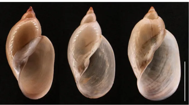
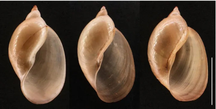
Figure 4.6: Shells of R. rubiginosa (Amatikulu) showing the variation found in the population, scale bar 10 mm...

Figure 4.7: Shells of L. natalensis (UKZN Pond) showing the variation found in the population, scale bar 10 mm...

Figure 4.8: Shells of L. natalensis (Greyville Pond) showing the variation found in the population, scale bar 10 mm...

Figure 4.9: Plot of canonical scores defined by functions 1 and 2 from forward stepwise DFA of shell morphological characters for size class 1 (shell length < 10 mm). Radix rubiginosa from the Amatikulu site is represented by the closed circles (●). Lymnaea natalensis from the UKZN Pond and Greyville Pond are indicated by the open triangles () and open squares (□) respectively...

Figure 4.10: Plot of canonical scores defined by function 1 and 2 from forward stepwise DFA of shell morphological characters for size class 2 (shell length ≥ 10 mm). Radix rubiginosa from the Amatikulu site is represented by the closed circles (●). Lymnaea natalensis from the UKZN Pond and Greyville Pond are indicated by the open triangles () and open squares (□) respectively...

Figure 4.11: Scanning electron micrograph of the central tooth and lateral teeth of R. rubiginosa. A smaller accessory cusp is located on the left side towards the base of the central tooth (indicated by the arrows), scale bar 3 μm.

Figure 4.12: Scanning electron micrograph of the lateral teeth from the left side of a transverse row of R. rubiginosa, scale bar 10 μm...

57

61

62

63

69

72

74

75

(28)

Figure 4.13: Scanning electron micrograph of the intermediate laterals (10^th and 11^th pairs of teeth) of R. rubiginosa. The 10^th pair was tricuspid but developed a small enlargement towards the base of the ectocone (indicated by the arrow). In the 11^th pair the ectocone, located towards the base of the tooth, split into two cusps, scale bar 10 μm.

Figure 4.14: Scanning electron micrograph of the marginal teeth of R. rubiginosa, scale bar 10 μm...

Figure 4.15: External features and pigmentation patterns of R. rubiginosa from the Amatikulu hatchery.

A – Dorsal view of animal with shell removed to show the mantle pigmentation pattern, scale bar 10 mm.

el – eye lobe; f – foot; t – tentacle; m – mouth; vc – visceral coil; vm – visceral mass...

Figure 4.16: Scanning electron micrograph of the central tooth and lateral teeth of L. natalensis (Greyville), scale bar 3 μm.

Figure 4.17: Scanning electron micrograph of the lateral teeth of L. natalensis (Greyville), scale bar 10 μm...

Figure 4.18: Scanning electron micrograph of the intermediate laterals (7^th and 8^th pair of teeth) of L. natalensis (Greyville), scale bar 10 μm.

Figure 4.19: Scanning electron micrograph of the marginal teeth of L. natalensis (Greyville), scale bar 10 μm...

76

77

78

81

82

83

84

(29)

Figure 4.20: External features and pigmentation patterns of L. natalensis (Greyville).

A – Dorsal view of animal with shell removed to show the mantle pigmentation pattern, scale bar 10 mm.

el – eye lobe; f – foot; t – tentacle; m – mouth; vc – visceral coil; vm – visceral

mass... 85

Chapter 5

Figure 5.1: Characteristic egg capsule morphology for the Lymnaeidae (A) and Physidae (B) showing curvature of the capsule after oviposition. Dextral and sinistral families have the egg capsules curved in opposite directions, R. rubiginosa and L. natalensis are dextral snails while P. acuta is a sinistral snail. Lymnaeid capsules display anticlockwise torsion while physid capsules show clockwise torsion. In lymnaeid capsules (C), distinct capsular strings and egg strings were observed, resulting in the characteristic corkscrew arrangement of the eggs within the capsule. In the Physidae (D), the egg strings were not as well developed as in the Lymnaeidae, scale bar 1 mm.

cs – capsular strings; e – egg; em – external membrane; et – existus terminalis (terminal point of capsule); fo – fila ovi (egg strings); im – internal membrane;

pg – pallium gelatinosum (gelatinous slimy outer envelope)...

Figure 5.2: Sequence of the morphological characteristics occurring during the first cleavage (2-cell stage).

A – Fertilised egg cell before cleavage.

B – Uncleaved egg cell showing the animal and vegetative poles, with the polar body (see arrow).

C – Cleavage was initiated at the animal pole by the appearance of a cleavage furrow (see arrow).

98

(30)

D – First cleavage divided the egg cell into blastomeres AB and CD. The blastomeres were linked to each other by the cytoplasmic bridge (see arrow).

E – The blastomeres approached each other, increasing their surface contact.

F – The cleavage cavity was observed between the two blastomeres.

ap – animal pole; cc – cleavage cavity; vp – vegetative pole...

Figure 5.3: During the cleavage period of rapid cell division, the size of the embryo does not change, rather the cleavage cells or blastomeres become smaller with each division. In second cleavage (4-cell stage), the four large blastomeres A, B, C and D were of the same size and orientated side by side.

The cleavage furrows linking the alternate blastomeres in the animal and vegetative poles of the embryo were observed. In addition the cleavage cavity (see arrow) reappeared in the central space formed by the furrows of the blastomeres.

This regular succession of formation and extrusion of the cleavage cavity continues until the gastrula stage...

Figure 5.4: Third cleavage (8-cell stage) showing an upper tier of micromeres (1a – 1d) and the lower tier of macromeres (1A – 1D). The micromeres were

orientated over the junction between each of the macromeres.

A – Lateral view of the 8 cell stage, showing the upper tier of micromeres and a lower tier of macromeres.

B – Third cleavage when viewed from the egg axis or from the animal pole. The cleavage cavity was observed in the animal half of the embryo.

cc – cleavage cavity; ma – macromeres; mi – micromeres...

Figure 5.5: The fourth cleavage (16-cell stage). During this stage, the dexiotropically-formed micromeres and marocmeres divided laeotropically.

cc – cleavage cavity; ma – macromeres; mi – micromeres...

Figure 5.6: At the fifth cleavage (24-cell stage), dexiotropic division of the embryo occurred...

109

111

112

113

114

(31)

Figure 5.7: During the sixth cleavage (64-cell stage), the micromeres and

macromeres divided laeotropically. Also, division synchrony was lost at this stage and bilaterally symmetrical division took place...

Figure 5.8: The blastula stage.

A – Embryo with space between the animal and vegetative poles.

B – Blastocoel surrounded by cells (see arrow).

bc – blastocoel...

Figure 5.9: During the gastrula stage, the macromeres situated in the centre of the vegetal region changed in shape. They reduced their external surface area whereas the inner part widened forming a pit at the vegetal pole of the embryo. At the beginning of the gastrula stage, this pit (blastopore) was very wide. As gastrulation proceeded, the blastopore narrowed and closed from back to front until only a small opening remained.

A – Young gastrula with a wide pit (blastopore) forming at the vegetative pole.

B – Older gastrula with a reduced blastopore.

ap – animal pole; bp – blastopore; vp – vegetative pole...

Figure 5.10: Trochophore embryo developed after gastrulation showing the prototroch, a band of ciliated cells, the prototroch, around the equator. The prototroch thus divided the trochophore into the upper pretrochal region and the lower posttrochal region. Smaller cilia also occurred over the rest of the larva. The blastopore moved towards the apical plate and developed into the mouth (see arrow).

lpt – lower posttrochal region; pr – prototroch; upt – upper pretrochal region...

Figure 5.11: Late trochophore showing development of the distinct anterior region and visceral mass, indicated by the accumulation of large vacuolated cells. The formation of the shell gland, represented by a thickening of the ectoderm (see arrow) occurred at the posterior region where the shell spire later develops. No

115

116

117

(32)

evidence of the shell was seen at this stage. During the late trochophore stage, the larva was still observed to move within the egg.

f – foot; sg – shell gland...

Figure 5.12: The early veliger stage showing the development of a distinct head, shell and foot.

A – The head region was distinguished with aggregations of ganglia forming the eyes (see arrow). The posterior region of the visceral mass was covered by an embryonic shell.

B – The embryo exhibited considerable coordination of movement by use of the muscular foot. Elevations of the tentacle regions were observed as well as a raised ridge marking the margin of the mantle (see arrow). This ridge encircled the lower part of the visceral mass.

f – foot; s – shell; t – tentacles; vm – visceral mass...

Figure 5.13: The late veliger embryo. The ridge (see arrow) marking the edge of the mantle clearly differentiated the visceral mass from the muscular foot region.

The shell was now larger and covered the entire visceral mass. At the anterior head region, the eyes were more prominent. The heart and other organs of the visceral mass were also visible.

e – eyes; f – foot; s – shell; vm – visceral mass...

Figure 5.14: Young snail shortly before hatching. The snail occupied the entire interior of the egg. Continued thinning of the internal egg membrane by the movements of the shell and foot resulted in its rupture.

e – eyes; f – foot; m – mouth; s – shell; vm – visceral mass...

118

119

120

121

(33)

Chapter 6

Figure 6.1: Growth expressed as an increase in the mean shell length for R.

rubiginosa, L. natalensis (UKZN and Greyville Ponds) and P. acuta at 20^oC (n = 90)...

Figure 6.4: The von Bertalanffy growth curve for R. rubiginosa, L. natalensis (UKZN and Greyville Ponds) and P. acuta at 20^oC...

Figure 6.7: Age specific survival rates (l_x) for R. rubiginosa, L. natalensis (UKZN and Greyville Ponds) and P. acuta at 20^oC...

Figure 6.8: Age specific survival rates (lx) for R. rubiginosa, L. natalensis (UKZN and Greyville Ponds) and P. acuta at 25^oC...

144

145

146

148

149

150

152

154

(34)

Figure 6.9: Age specific survival rates (lx) for R. rubiginosa, L. natalensis (UKZN and Greyville Ponds) and P. acuta at 30^oC...

Figure 6.10: Age specific fecundity (m_x) for R. rubiginosa, L. natalensis (UKZN and Greyville Ponds) and P. acuta at 20^oC...

Figure 6.11: Age specific fecundity (mx) for R. rubiginosa, L. natalensis (UKZN and Greyville Ponds) and P. acuta at 25^oC...

Figure 6.12: Age specific fecundity (m_x) for R. rubiginosa, L. natalensis (UKZN and Greyville Ponds) and P. acuta at 30^oC...

156 158

161

163

(35)

________________________________________________________________________

1

General Introduction

________________________________________________________________________

1.1 Biological Invasions

Anthropogenic alterations of natural ecosystems and human-assisted dispersal of species outside of their native ranges have caused an unprecedented redistribution and

homogenization of the Earth’s biota (Olden et al., 2004). The expansion of a species range is a natural process, but non-indigenous introductions are growing increasingly frequent as species are moved across geographical barriers, either intentionally or unintentionally (Perrings et al., 2000; Ricciardi, 2006).

The process of invasion can be divided into three successive stages namely; introduction, establishment and integration. Introduction involves the dispersal of a non-indigenous species from its native range to that of the recipient range. Through local reproduction and recruitment the new population is established (Vermeij, 1996; Richardson et al., 2000). This would eventually augment or replace dispersal from the native range as a means for the sustainability of the invading population. Integration occurs when the invading species develops ecological links with other species in the recipient region (Vermeij, 1996; Richardson et al., 2000).

Although research on biological invasions is often weighted toward terrestrial ecosystems, the importance of understanding and preventing non-indigenous species introductions in aquatic systems is highlighted by the increasing number and rate of freshwater invasions, the high endemicity of freshwater ecosystems and the importance of freshwater ecosystems for human health and the economy (Johnson et al., 2009).

Considering that freshwater covers only about 0.8% of the Earth’s surface (Gleick, 1996),

(36)

vulnerable to non-indigenous species introductions. Since abiotic conditions in freshwater ecosystems are generally more homogenous and less fluctuating than in terrestrial habitats (Cohen and Carlton, 1998; Padilla and Williams, 2004; Gollash, 2006), the initial chances of survival for an aquatic non-indigenous species may be higher

(Cook, 1990). Once introduced into an ecosystem, dispersal (either intentional or

unintentional) may be easier for freshwater than terrestrial species. This is expected since fewer dispersal barriers exist for freshwater ecosystems.

Pathways of intentional introduction for freshwater species are the trades in live aquatic organisms including aquaculture (Naylor et al., 2001), nursery plants (Reichard and White, 2001; Maki and Galatowitsch, 2004), live food (Weigle et al., 2005), pet (Padilla and Williams, 2004; Rixon et al., 2005) and bait trades (Mills et al., 1993). Other pathways arise for the unintentional transfer of freshwater species. These include transport in ballast tanks of intercontinental ships (Mills et al., 1993; Ricciardi, 2006), inter-basin and inter-catchment transfer schemes for water supply purposes and introduction as contaminants of aquatic plants (Maki and Galatowitsch, 2004).

1.2 Factors affecting Biological Invasions

In general, the species that become successful invaders are predicted to be species that, in their native ranges, display traits that prompt them to successfully survive conditions encountered during transport, introduction, establishment and integration (Suarez and Tsutsui, 2008). Two main attributes of biological invasions are: invasiveness, i.e. the traits that enable a species to invade a habitat and invasibility, i.e. the characteristics of the new habitat that determine its susceptibility to the establishment and integration of an invasive species (Lonsdale, 1999; Alpert et al., 2000; Marco et al., 2002).

Successful invaders possess characteristics associated with effective dispersal, rapid growth, short generation times, high fecundity, a high degree of phenotypic plasticity, broad physiological tolerance (euryhalinity and eurythermy) and a broad diet (Rejmanek

(37)

and Richardson, 1996; Williamson and Fitter, 1996; Reid and Orlova, 2002; Ruesink, 2005; Moyle and Marchetti, 2006; Keller et al., 2007; Suarez and Tsutsui, 2008).

Also, the abiotic environment sets clear limits on species invasibility. Invasion site characteristics hypothesized to favour frequent or rapid invasion include (a) similarity to the native ranges of the invasive species, (b) a history of recent natural or anthropogenic disturbance, and (c) a low niche diversity within the habitat (Elton, 1958; Moyle and Light, 1996; Moyle and Marchetti, 2006). It should be noted though that caution must be taken when using such characteristics for predicting invasions as each invader uses the biotic and abiotic environment in a different way.

1.3 Impacts of Biological Invasions

While not all introduced species become invasive, successful colonisers can have major ecological, economic and health implications. Ecological impacts are focused on faunal composition, community structure and ecosystem functioning (Mack et al., 2000). All these impacts are mediated by numerous processes that act at the individual, community and ultimately the ecosystem level (Simon and Townsend, 2003). At the level of the individual, invasive species may alter the behaviour of indigenous species, influencing habitat use and foraging. At the population level, the invasive species may influence changes in the abundance or distribution of other species. According to both Gurevitch and Padilla (2004) and Ricciardi (2004), the introduction of non-indigenous species acts as a significant driver of global biodiversity loss, second only to habitat destruction.

These changes in or even loss of biodiversity may occur through predation, competition, hybridization with the indigenous species, extirpation of competitively inferior species and alteration of the abiotic environment (Vitousek et al., 1996; Ricciardi et al., 1998;

Mack et al., 2000; Clavero and Garcia-Berthou, 2006). At the community level, invaders may alter both direct and indirect interactions among populations and finally, at the ecosystem level invasive species may change the pathways and magnitude of movements of energy and nutrients (Simon and Townsend, 2003).

(38)

Economic impacts result from the effects of introduced species on the indigenous biota, as well as funds expended for costly control or eradication programmes (Perrings et al., 2000). Introduced species have also affected industrial constructions such as reservoirs, pumps and water pipes. For an example, in the United States, it is estimated that non- indigenous species cost the national economy $120 billion to $137 billion per year (Pimentel et al., 2005), while for the United Kingdom, Australia, South Africa, India and Brazil together, costs exceeded $200 billion (Pimental et al., 2001). Finally, invasive species can impact human health either directly when they are infectious or pathogenic to humans, or indirectly by promoting the transfer of disease.

1.4 Invasive freshwater snails in South Africa

In an assessment of the ecological impact and economic consequences of invasive freshwater snails in South Africa, Appleton (2003) listed a prosobranch (Tarebia granifera Lamarck, 1822) and three pulmonates (Lymnaea columella Say, 1817, Physa acuta Draparnaud, 1805 and Aplexa marmorata Guilding, 1828) as being of concern.

Lymnaea columella and P. acuta were introduced in the early 1940s (Brown, 1994;

Appleton and Brackenbury, 1998; Appleton, 2003), while A. marmorata was collected for the first time in this country in 1986 (Appleton et al., 1989). The recently introduced species, T. granifera, was reported for the first time in Africa by Appleton and Nadasan (2002) after it was discovered in 1999 in a reservoir supplying water to a paper mill in KwaZulu-Natal.

1.5 First Report of Radix rubiginosa in South Africa

In 2004, a large population of an unknown lymnaeid was found in a prawn and tropical fish breeding facility in Amatikulu, northern KwaZulu-Natal, South Africa. Since Asia is a frequent source of supply for tropical fish and plants for the South African aquarium trade, and the fact that several other snails in this facility were of Asian origin, it was thought likely that this new lymnaeid was Asian as well. Available keys to Asian freshwater snails (Brandt, 1974; Burch, 1980) suggested that the new snail belonged to

(39)

the genus Radix but could be any of several species known from the region. In 2007 snails supplied by myself from the Amatikulu Hatchery were identified using molecular techniques as Radix rubiginosa (Michelin, 1831) – a species widespread in southeast Asia (J. Lamb and K. Pillay, unpubl. data).

Radix rubiginosa has been listed as a “hothouse” alien species in Great Britain, Ireland and Israel (Mienis 1986; Anderson, 2005), becoming established in greenhouses, aquaria within greenhouses and similar artificially-heated habitats. Dondero and Lim (1976) and Mienis (1986) have commented that it is easy to breed R. rubiginosa in aquaria and this was also found to be the case in this study. The indigenous Lymnaea natalensis Krauss, 1848 is not as easy to breed and this raises the question, “If R. rubiginosa spreads in South Africa, will it do so at the expense of L. natalensis?” The natural occurrence of L.

natalensis in KwaZulu-Natal appears to have decreased already perhaps due to the invasiveness displayed by yet another lymnaeid, Lymnaea columella. If R. rubiginosa populations become established in the same area then this could increase pressure on the indigenous L. natalensis and eventually lead to its extirpation (C.C. Appleton pers.

comm.).

The presence of R. rubiginosa in a nearby reservoir on the Amatikulu facility, suggests that the spread of this species may already have taken place. Furthermore, accidental escape or deliberate release may well go unnoticed due to its strong resemblance to the indigenous L. natalensis. This is because the shell morphology of L. natalensis is notoriously variable and some of its variants resemble R. rubiginosa. There was thus a clear need to be able to differentiate the two lymnaeid species but identification was difficult due to unclear and contradicting accounts in the literature. This is further complicated by increasing evidence suggesting that the forms of what is widely called L.

natalensis in Africa may in fact comprise more than one species (Brown, 1994).

Snails introduced into new settings provide opportunities for new host-parasite

associations to develop and according to Mas-Coma and Bargues (1997), a broad range of lymnaeid species can serve as hosts of fasciolid parasites. In South Africa, the

(40)

intermediate host of the giant liver fluke Fasciola gigantica is Lymnaea natalensis and this fluke is confined to the subtropical lowland regions. The intermediate host for the common liver fluke Fasciola hepatica is Lymnaea truncatula Müller, 1774, however this species is confined to the cooler areas of the eastern highlands in South Africa (altitude above approximately 800 m), and also the low-lying parts of the Eastern and Western Cape, South Africa (Brown, 1994). Radix rubiginosa serves as the intermediate host for F. gigantica over much of south-eastern Asia (Srihakim and Pholpark, 1991; Malone, 1997) and if it were to become invasive in South Africa, it could exacerbate the fascioliasis problem in the country. Radix rubiginosa has also been identified as the intermediate host for the avian blood fluke, Trichobilharzia sp., a cause of schistosome dermatitis (Nithuithai et al., 2004), Schistosoma incognitum (Bunnag et al., 1983) and various echinostomes (Charoenchai et al., 1997).

The overall aim of this study was to assess the invasive capability of R. rubiginosa in South Africa. By comparing specific characteristics between R. rubiginosa and the already invasive North American snail Physa acuta (Physidae), it was possible to assess the potential impact of this introduced lymnaeid on the indigenous L. natalensis.

This study is arranged in seven chapters. Chapter 1 provides an overview of the literature on biological invasions giving emphasis on factors affecting invasion, as well as the possible or proven impacts of such invasions.

Chapter 2 provides a review of the family Lymnaeidae. In this Chapter the phylogeny of the Lymnaeidae is addressed based on conchological, anatomical and molecular

characteristics.

Invasion by R. rubiginosa is likely to go unnoticed because the shell morphology of L.

natalensis is highly variable and some of its variations resemble those of R. rubiginosa.

There was thus a clear need to be able to differentiate the two lymnaeid species but identification was difficult due to a lack of clarity in the literature. Chapter 3 presents a

(41)

redescription of the indigenous species L. natalensis with emphasis on conchological and anatomical characters.

In Chapter 4, the traditional morphometric approach was used to assess the suitability and efficacy of conchological characters to distinguish shell variations and patterns within and between populations of two species of Lymnaeidae, the introduced R. rubiginosa and the indigenous L. natalensis. This includes an examination of the radula, the

reproductive anatomy and a description of the pigmentation patterns on the mantle.

These characters were then used as criteria to easily recognize and separate R. rubiginosa from L. natalensis.

Chapter 5 describes and compares the effects of three experimental temperatures on the hatching rates and embryonic development of four populations of three snail species: R.

rubiginosa from the Amatikulu Hatchery, L. natalensis from both the UKZN and

Greyville Ponds and P. acuta from the Greyville Pond. A description of the morphology of each developmental stage is provided. In addition, a study of the frequency of various egg abnormalities and their relation to the breeding intensity of these species are

assessed.

In Chapter 6 the invasiveness of R. rubiginosa is assessed in relation to the indigenous L.

natalensis and the already established invader, the North American, Physa acuta. This investigation determined the growth, survivorship, fecundity and life history parameters of the three species and the role of temperature in causing observed differences. This was seen as particularly important in view of the success of P. acuta as an invader in South Africa. The growth, survivorship, fecundity and life history parameters were then comparatively analysed to allow for a more precise focus on the specific attributes that may determine the invasive success of R. rubiginosa.

Chapter 7 presents a general discussion of the present study, integrating the key findings and conclusions from the previous chapters.

(42)

________________________________________________________________________

2

Review of the Family Lymnaeidae

________________________________________________________________________

The pulmonate basommatophoran superfamily Lymnaeoidea includes several families of freshwater snails, among which is the Lymnaeidae. The Lymnaeidae inhabit a wide variety of freshwater habitats, and as such display a tremendous morphological diversity, both conchological and anatomical. This high level of morphological diversity makes phylogenetic studies of the Lymnaeidae difficult. Despite this, interest in phylogeny of the lymnaeids is important, because firstly, many lymnaeid species are intermediate hosts for trematode parasites and secondly, lymnaeids are part of a growing number of

freshwater taxa that are threatened due to the increasing destruction of freshwater ecosystems.

2.1 The systematic – taxonomic confusion in the family Lymnaeidae

About 1800 species and 34 genera of lymnaeids have been named in the past, with classifications recognising a single genus (Walter, 1968), two genera (Hubendick, 1951;

Te, 1976; Jackiewicz, 1998) or more than two genera (Burch, 1965, 1980; Malek, 1985;

Jackiewicz, 1993; Glöer and Meier-Brook, 1998), while Kruglov and Starbogatov (1993) recognised up to 26 different genera within the family.

Despite several approaches being used to evaluate the taxonomy and relationships within the family, consensus has not yet been reached because of the poor/inadequate systematic resolution of the information (Hubendick, 1951; Burch, 1965; Inaba, 1969; Walter, 1969;

Burch and Lindsay, 1968; Burch and Ayers, 1973; Rudolph and Burch, 1989; Remigio and Blair, 1997). Disagreement between the results of morphological studies on the shell, radula and prostate gland with those from karyological and biochemical methods

(43)

(Bargues et al., 2001), suggests that morphological and anatomic homoplasy is common among lymnaeids. Hence species systematics and delineation within the Lymnaeidae are obscure due to the great number of described species and the morphological similarities between them. These have often made identification of specimens of the Lymnaeidae difficult (Mas-Coma and Bargues, 1997).

2.2 Phylogeny of the Family Lymnaeidae

The phylogeny and classification of the Lymnaeidae has traditionally been based on the use of shell characters, however, once the variable nature of the shell was demonstrated, workers started to take a more anatomical focus in species determination. In recent years, various cytological, biochemical and molecular studies ha