Investigation of the relationship between solar radiation and cloud cover using a total sky imager.

(1)

Investigation of the relationship between solar radiation and cloud cover using a Total Sky Imager

by

Elison Soul Ganya

Submitted in fulfilment of the academic requirements for the degree of Master of Science in the School of Chemistry and Physics,

University of KwaZulu-Natal, Durban March 2017

(2)

ii

Abstract

Solar radiometric studies have been done in South Africa, but no research studies have been performed to understand how the cloud fraction (CF) affects the amount of solar radiation received by radiometers. This work focused on studying the relationship between radiometry readings and cloud fraction at the University of Kwa-Zulu Natal (UKZN) at Howard College in Durban. This study used a pyrheliometer to measure beam irradiance (DNI), a shaded pyranometer to measure diffuse irradiance (DHI), an unshaded pyranometer to measure global irradiance (GHI) and a Total Sky Imager to give CF percentage. When we studied 1- minute data of radiometric profiles versus CF with respect to time, we found that an increase in CF resulted in a decrease in DNI except for the rare moments when the clouds did not obstruct the sun. An increase in CF resulted in an increase in DHI only if the sky was not overcast. For an overcast sky, there is no simple relationship between CF and DHI. When we studied centred moving averages of DNI against clearness fraction (1 – CF) as a function of time for different time-averaging scales, it was found that DNI had strong linear correlation with 1 – CF. When we studied centred moving averages of DHI and CF as a function of time for different averaging scales, it was found that DHI increased as CF increased but only if the sky was not overcast. Scatter plots of different clearness indices against CF for different averaging scales were studied and it was found that linear correlation increased with averaging scale, and beam-related clearness indices had a strong linear relationship with CF at a time-averaging scale of 4 hours.

(3)

iii

Preface

The experimental work described in this dissertation was carried out in the School of Chemistry and Physics, University of KwaZulu-Natal, Westville, Durban, from January 2013 to April 2015, under the supervision of Dr. A.P. Matthews and Professor Sivakumar Venkataraman. These studies represent original work by the author and have not otherwise been submitted in any form for any degree or diploma to any tertiary institution. Where use has been made of the work of others, it is duly acknowledged in the text.

(4)

iv

Declaration-Plagiarism

I, Elison S. Ganya declare that

1. The research reported in this thesis, except where otherwise indicated, is my original research.

2. This thesis has not been submitted for any degree or examination at any other university.

3. This thesis does not contain other persons' data, pictures, graphs or other information, unless specifically acknowledged as being sourced from other persons.

4. This thesis does not contain other persons' writing, unless specifically acknowledged as being sourced from other researchers. Where other written sources have been quoted, then:

(a) Their words have been re-written but the general information attributed to them has been referenced.

(b) Where their exact words have been used, then their writing has been placed in italics and inside quotation marks, and referenced.

5. This thesis does not contain text, graphics or tables copied and pasted from the Internet, unless specifically acknowledged, and the source being detailed in the thesis and in the Bibliography section.

Signed: . . .

(5)

v

Acknowledgements

Firstly, I would like to thank my supervisor Dr A.P Matthews for his unwavering support, motivation and kind supervision during the entire period of my research. You so understood and were patient with me. I would like to thank my co-supervisor Professor Sivakumar Venkataraman for his advice during the course of this research project.

I am also indebted to thank the Principal Technician, Enock Chekure for his support and assistance throughout the entire period of my research. I am grateful for your help and patience when dealing with my requests. Special thanks to my colleague Paulene Govender for her assistance, advice and unwavering support in making this project successful.

To the staff at Howard College, Mike Brooks and his team, I would like to thank you for your assistance in maintaining the radiometry and TSI equipment.

Great thanks to my friend Dr Mhlambululi Mafu for his support and guidance during the course of this research project.

Lastly, I would like to thank my wife and family for all their encouragement and unconditional support.

(6)

vi

List of Figures

Figure 1.1: Average daily DNI for South Africa for the entire year . ... 3 Figure 2.1: Structure of the sun ... 22 Figure 2.2: The atmosphere affects the amount and distribution of solar radiation reaching the ground . ... 24 Figure 2.3: Interaction of incoming Solar Radiation with the atmosphere and ground . ... 25 Figure 2.4: Sketches of the angular pattern of the scattered intensity from particles of various sizes . ... 27 Figure 2.5: AM: Air Mass index . ... 28 Figure 2.6: Scattering of the direct-beam photons from the sun by the atmosphere produces diffuse radiation that varies with AM . ... 29 Figure 2.7: Radiation balance of the atmosphere ... 30 Figure 2.8: Scattering of the direct-beam photons from the sun by the atmosphere ... 31 Figure 2.9: Position of the equinoxes, solstices, aphelion, and perihelion relative to the Earth's orbit around the Sun . ... 34 Figure 3.1: Angstöm pyrheliometer (a) external view, (b) schematic of the instrument, (G1) and (G₂) galvanometers, (R) rheostat regulating the strength of the compensation current ... 39 Figure 3.2: Silver-disk pyrheliometer . ... 40 Figure 3.3: Cross section of the Eppley NIP ... 41 Figure 3.4: Pyrheliometer mounted onto the Solys 2 tracker measures the DNI component. . 43 Figure 3.5: Thermo-electric pyranometer . ... 44 Figure 3.6: Bimetallic pyranograph . ... 45 Figure 3.7: Shaded and unshaded pyranometers mounted on a stationary plate on top of the Solys 2 tracker... 46 Figure 3.8: Clear-Sky Image (left end), Corresponding Relative Red/Blue Ratio Image, (second from left end), Separated Blue (second from right end), and Red (right end) Pixel Value Amount Images. ... 51 Figure 3.9: Cloud Detection Image Corresponding to Fig 3.3. Black denotes masking. Green outlines denote areas where separate cloud/clear pixel counts are included in the sky cover

(10)

x

retrieval output files. Cloud detection color scheme is clear (blue), thin cloud (gray) and

opaque cloud (white) ... 52

Figure 3.10: Cloudy-Sky Image (left end), Corresponding Relative Red/Blue Ratio Image (second from left end), Separated Blue (second from right end), and Separated Red (right end) Pixel Value Amount Images . ... 53

Figure 3.11: Cloud Detection Image Corresponding to Fig 3.5. Black denotes masking. Green outlines denote areas where separate cloud/clear pixel counts are included in the sky cover retrieval output files. Cloud detection color scheme is clear (blue), thin cloud (gray) and opaque cloud (white) ... 53

Figure 3.12: Model TSI-440 Total Sky Imager as mounted on Desmond Clarence Building, at UKZN Howard College Campus, Durban. ... 55

Figure 3.13: Processed image (left) and Raw sky image (right) at time 10:52 on the 01^st of October 2014. ... 56

Figure 3.14: Processed image (left) and Raw sky image (right) at 11:45 on 14^th of July 2014. The CF was 41% and the sky condition was sunny... 57

Figure 4.1: Instrument setup at the test site of the radiometric instruments (pyrheliometer and shaded and unshaded pyranometers) and TSI connected to CR1000 data logger. ... 61

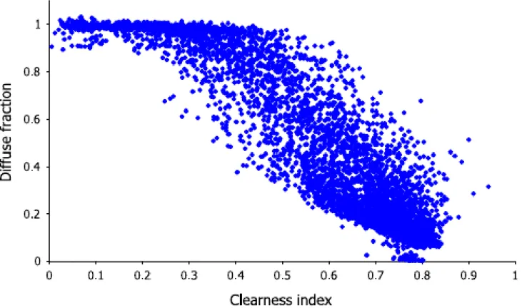
Figure 4.2: Plot of diffuse fraction kd against clearness index kt for 1-minute data at Eugene . ... 63

Figure 4.3: Graph of the kd against clearness index kt for 1-minute data of the entire dataset. ... 64

Figure 4.4: Plot of k_b versus k_t for 1-minute data at Eugene . ... 65

Figure 4.5: Graph of k_b vs k_t for 1-minute data of the entire data. ... 65

Figure 4.6: Graph of clear sky and actual radiometric readings for 04 December 2014. ... 67

Figure 5.1: Raw sky image (a) and processed image (b) at 11:09 on 14^th of July 2014. The CF was 4% and the sun was not obstructed by clouds. ... 70

Figure 5.2: Plot of CF and solar irradiance against time between 06:00 and 18:00 on 14^th of July 2014. ... 70

Figure 5.3: Raw TSI image (a) and processed TSI image (b) at 11:45 on 14^th of July 2014. The CF was 41% and the sun was not obstructed. ... 71

Figure 5.4: Raw sky image (a) Processed image (b) and at 12:00 on 27^th of January 2015. The CF was 100% and the sun was obstructed by clouds. ... 72

Figure 5.5: Plot of CF and solar irradiance against time between 06:00 and 18:00 on 27^th of January 2015. ... 73

(11)

xi

Figure 5.6: Raw sky image (a) and processed image (b) at 13:03. The CF was 100% and the sky condition was not sunny. ... 74 Figure 5.7: Raw sky image (a) Processed image (b) and at 11:38 on 30^th of January 2015. The CF was 53% and the sun was obstructed by clouds. ... 75 Figure 5.8: Plot of CF and solar irradiance against time between 06:00 and 18:00 on 30^th of January 2015. ... 76 Figure 5.9: Plot of CF and solar irradiance against time between 06:00 and 18:00 on 30^th of January 2015. ... 76 Figure 5.10: Raw sky image (a) and processed image (b) at 08:25. The CF was 98% and the sky condition was sunny. ... 77 Figure 5.11: Plot of CF and solar irradiance against time between 11:00 and 13:00 on 30^th of January 2015. ... 78 Figure 5.12: Raw sky image (a) and processed image (b) and at 08:25. The CF was 71% and the sky condition was sunny. ... 79 Figure 5.13: Raw TSI image at (a) 10:00 (b) 11:00 and (c) 12:00. Processed TSI image at (d) 10:00 (e) 11:00 and (f) 12:00. ... 79 Figure 5.14: Plot of CF and solar irradiance against time between 06:00 and 18:00 on 10^th of September 2014. ... 80 Figure 5.15: Plot of CF and solar irradiance against time between 10:00 and 12:00 on 10^th of September 2014. ... 81 Figure 5.16: Processed 1-minute images between 10:16 to 10:30 (from left to right on the top row and down row also from left to right). The CF increased from 71% at 10:16 to 100% at 10:30. The temporal variation of images shows cloud evaluation from South East direction. 82 Figure 5.17: Raw sky image (a) and processed image (b) at 11:56. The CF was 97% and the sun was not obstructed. ... 83 Figure 5.18: Plot of centred moving average DNI and 1 – CF against time for different time- averaging time-scales τ ... 86 Figure 5.19: Plot of centred moving average DHI and 𝐶𝐹 against time for different time- averaging time-scales τ ... 88 Figure 5.20: Scatter plot of k_t as a function of the total CF for the entire I minute dataset. .... 90 Figure 5.21: Scatter plot of k_c as a function of the total CF for the entire 1 minute dataset. ... 91 Figure 5.22: Scatter plot of k_b against CF for the entire I minute dataset. ... 92 Figure 5.23: Scatter plot of DNI/DNI_c as a function of the total CF for the entire 1 minute dataset. ... 93

(12)

xii

Figure 5.24: Scatter plot DHI/DHI_c as a function of the total CF for the entire 1 minute

dataset. ... 94

Figure 5.25: Scatter plot of k_t as a function of the total CF for the entire dataset. ... 95

Figure 5.26: Scatter plot of k_c as a function of the total CF for the entire dataset. ... 96

Figure 5.27: Scatter plot of k_b as a function of the total CF for the entire dataset. ... 97

Figure 5.28: Scatter plot of DNI/DNI_c as a function of the total CF for the entire dataset. ... 98

Figure 5.29: Scatter plot of DHI/DHI_c as a function of the total CF for the entire dataset. .... 99

Figure 5.30: Scatter plot of k_t as a function of the total CF for the entire dataset. ... 100

Figure 5.31: Scatter plot of kc as a function of the total CF for the entire dataset. ... 101

Figure 5.32: Scatter plot of kb as a function of the total CF for the entire dataset. ... 102

Figure 5.33: Scatter plot of DNI/DNIc as a function of the total CF for the entire dataset. ... 103

Figure 5.34: Scatter plot of DHI/DHIc as a function of the total CF for the entire dataset. .. 104

Figure 5.35: Scatter plot of kt as a function of the total CF for the entire dataset. ... 105

Figure 5.36: Scatter plot of kc as a function of the total CF for the entire dataset. ... 106

Figure 5.37: Scatter plot of kb as a function of the total CF for the entire dataset. ... 107

Figure 5.38: Scatter plot of DNI/DNIc as a function of the total CF for the entire dataset. ... 108

Figure 5.39: Scatter plots of DHI/DHIc as a function of the total CF for the entire dataset. . 109

Figure B.1: KZH station details. ... 131

Figure D.1: Scatter plots for 30 minutes average ... 133

Figure D.2: Scatter plots for 2 hours average ... 134

Figure D.3: Scatter plots for 3 hour average ... 135

(13)

xiii

List of Tables

Table 2.1: The day N corresponding to the i-th day of the month ... 35 Table 6.1: Correlation coefficient and coefficient of determination for clearness indices against CF ... 115 Table A.1: Nomenclature ... 128

(14)

1

Chapter 1 Introduction

The world still depends much on the carbon sources of energy which are having negative environmental impact such as global warming. The burning of fossil fuels emits greenhouse gases such as CO2 and methane (CH4) which absorb long-wave solar radiation, preventing it from leaving the earth's atmosphere and entering into space. This results in excess thermal energy being trapped in the atmosphere because the greenhouse gases emit the absorbed long- wave radiation raising the temperature of the earth. This process is known as global warming (Kalogirou, 2004). In order to reduce the effects of global warming, there must be a decrease in the pollution created by power plants and automobiles that involve burning of fossil fuels and more environmentally friendly energy alternatives have to be utilised. Apart from the negative environmental impact, the rate at which the carbon sources are depleted is of great concern since it is not renewable. This gave birth to the idea of utilising free renewable energy sources.

Environmentally friendly energy sources include solar, wind, hydro, biofuel and geothermal.

Solar energy stands out as the most abundant energy resource on Earth. However, harnessing this form of energy optimally is still a challenge. Solar energy is used in photovoltaics (PV) and solar thermal system (STS) which are concentrating or non-concentrating. These two are primary forms of electricity generation. Sunlight is the fuel for all PV’s and STS’s generation technologies. The performance of the PV’s and STS’s at any place depends on the available insolation as well as other meteorological parameters. Insolation is the measure of solar radiation that is received at a specific location and time, commonly expressed as average irradiance in W/m² (Rudd, 2011). Proper understanding and thorough knowledge of the available insolation reaching a site is important for accurate analysis of system performance and financial viability of a project on a site ( Stoffel, et al., 2010).

(15)

2

South Africa has an average annual Direct Normal Irradiation (DNI) of more than 2500 kWh/m² which fortunately makes it one of the best solar resourced countries in the world (Edkins, Winkler, & Marquard, 2009). Direct Normal Irradiance (DNI) is the amount of solar radiation received per unit area by a surface that is always held perpendicular (or normal) to the rays that come in a straight line from the direction of the sun at its current position in the sky (solargis).

The high average DNI for South Africa make it an ideal location for implementing solar powered technologies. Fig 1.1 illustrates the DNI distribution for South Africa. KwaZulu-Natal province is one of the areas with the lowest annual average DNI of less than 6.0 kWh/m²/d. The Northern Cape has the highest DNI of more than 7.0 kWh/m²/d, which make it an appropriate location for implementing concentrated solar power (CSP) technologies (Fluri, 2009).

(16)

3

Figure 1.1: Average daily DNI for South Africa for the entire year (Fluri, 2009).

(17)

4

Clouds have an effect on the radiation received at the earth's surface and this knowledge is vital for a radiative energy budget. Amongst other factors, clouds are the primary source of solar radiation fluctuation (Peng, Yoo, Yu, Huang, Kalb, & Heiser, 2014). Clouds are believed to reduce the available received radiation on the ground especially under overcast conditions (Josefsson & Landelius, 2000) (Renaud, Staehelin, Fröhlich, Philipona, & Heimo, 2000).

However, they are also believed to cause radiation levels exceeding the expected clear-sky value (also referred to as enhancements) on the received radiation on the earth’s surface if they are thin clouds (Pfister, McKenzie, Liley, Thomas, Forgan, & Long, 2003) (Sabburg & Wong, The effects of clouds on enhancing UVB irradiance at the Earth's surface:A one year study., 2000a) (Estupiñán, Raman, Crescenti, Streicher, & Barnard, 1996) (Weihs, Webb, Hutchinson, &

Middleton, 2000) (Schafer, Saxena, Wenny, Barnard, & DeLuisi, 1996). Enhancements may be due to both thick clouds (that scatter radiation) and due to thin clouds (that obscure the direct radiation). Thick clouds absorb radiation, but they can also scatter radiation from their sides, so that some extra radiation gets to the radiometers resulting in enhancement. Thin clouds will scatter the radiation so that much of it it becomes diffuse rather than direct and this effect results in enhancement. Cloud fraction (CF) is the fraction of the sky covered by clouds. The term cloud cover, cloud fraction and sky cover are being used interchangeably in this text since sky cover is also the fraction of cloud cover provided as a fraction between 0 and 1 (Parisi, Sabburg, Turner,

& Dunn, 2007). As mentioned above, cloud cover is a macro-physical aspect, but it is not the only aspect that affects the solar radiation, but micro-physical properties also do affect the solar radiation. However, in this section, we will focus more on how the cloud cover affects the solar radiation reaching the earth’s surface of the Durban area.

A Total Sky Imager (TSI) is an instrument that is used to map and measure cloud cover. This instrument can be used in conjunction with the pyranometer and pyrheliometer in order to predict the relationship between the cloud cover and the available solar radiation reaching the ground. A pyrheliometer is an instrument that is used to measure the direct normal irradiance (DNI) or direct solar radiation flux at normal incidence (Garg & Garg, 1993). A pyranometer is used to measure the global horizontal irradiance (GHI) and diffuse horizontal irradiance (DHI) that is

(18)

5

incident on them within the solid angle (Garg & Garg, 1993). Diffuse horizontal irradiance (DHI) is defined as the solar radiation received from the sun after its direction has been changed by scattering by the atmospheric constituents (Duffie & Beckman, 2013). Generally it is the scattered solar radiation from the sky dome (not including DNI). Global horizontal irradiance (GHI) is the geometric sum of the DNI and DHI (total hemispheric irradiance). The term

‘‘global’’ is associated with the fact that the solar radiation is received from the entire 2π solid angles of the sky vault (Paulescu, Paulescu, Gravila, & Badescu, 2013).

1.1 Research aim

The aim of this research is:

 To explain how cloud cover affects solar radiation measurements using a Total Sky Imager and radiometers in the Durban area.

1.2 Research question

 To what extent are direct and diffuse radiation a function of cloud cover, and over what time period?

1.3 Brief history of Sky Imagers (SIs)

Traditionally, the sky conditions were reported by specially trained human observers resulting in significant discrepancies due to the subjectivity in observations (Silva & Echer, 2013). Human observers were costly to maintain hence the manufacture of radiometry instruments (Long, Sabburg, Calbo, & Pages, Retrieving cloud characteristics from ground-based daytime color allsky images, 2006). There are many devices that can be used to automatically detect and quantify cloud amount and classify their type optically as in thin, thick or opaque. Satellite information can be used to get cloud information, but because of their weakness in quantifying small and/or low cloud features due to their limited spatial and temporal resolution they are rarely used (Long, Sabburg, Calbo, & Pages, Retrieving cloud characteristics from ground-based daytime color allsky images, 2006). In order to obtain continuous information on cloud cover, sky-imaging devices are used. Due to improvements in technology in recent years, there has been an increased development of ground-based sky imagers (Long, Sabburg, Calbo, & Pages, Retrieving cloud characteristics from ground-based daytime color all-sky images., 2006). However a Total Sky

(19)

6

Imager is the most common sky imager used in the research industry. More information on the Sky imagers is given in Chapter 3.

1.4 Literature review

There are mostly two methodologies that are commonly used for analysing cloud impacts which are namely hypothetical and experimental (Calbo, Pages , & Gonzalez , 2005). Hypothetical methodologies include the utilisation and improvement of radiative exchange hypothesis representing the impact of cloud particles on UV. Bead size dispersion and thickness or optical thickness and effective radius are then again the most critical physical variables that are utilised to depict water mists. Observational methodologies utilise a technique to recreate cloudless radiation and recognize the cloud impact by looking at the contrasts between measured radiation in overcast conditions and the assessed radiation in cloudless condition. Cloud impacts are concluded from the deliberate radiation in overcast conditions when contrasted with the cloudless model in which cloud impacts cannot be clarified like decreases and upgrades (Calbo, Pages , & Gonzalez , 2005). Calbo et al. (2005) investigated the exact phenomenon of cloud impacts on UV radiation over Spain. They particularly investigated the relationship between measured UV radiations in shady condition by fundamentally looking at the accompanying two strategies (Calbo, Pages , & Gonzalez , 2005):

 Techniques that include perception of cloud amount by people or using sky cameras.

 Techniques that utilize radiometric estimations as a substitute for cloud perceptions.

The cloud adjustment variable (CMF) is the proportion between the deliberate UV irradiance in overcast sky conditions and an expected cloudless UV irradiance (Staiger, den Outer, Bais, Feister, Johnsen, & Vuilleumier, 2008). Calbo et al. (2005) thought about after-effects of various works through figuring of CMF, which changes from 0.3 to 0.7 for cloudy skies relying upon cloud type and attributes. Cloud impact on UV radiation is 15 to 45% lower than on the total solar radiation. It was found that generally clouds have a reducing effect, whereas sometimes it has an enhancing effect on the downwelling radiation. Downwelling radiation is defined as the component of radiation directed toward the Earth’s surface from the sun or the atmosphere (Pfister, McKenzie, Liley, Thomas, Forgan, & Long, 2003).

(20)

7

Pfister et al. (2003) noticed enhancements in global irradiance for the most part happen on brief time scales; they tend not to be seen in information streams for which the mean irradiance is ascertained utilising a transient window of more than a couple of minutes (Pfister, McKenzie, Liley, Thomas, Forgan, & Long, 2003). In their work, they found that the enhancements in the global irradiance are connected with practically zero decrease in the beam irradiance and an expansion in the diffuse component part. The cloud fields in charge of enhanced surface irradiance do not basically lessen the beam irradiance but they increase scattering thereby increasing the diffuse component (Pfister, McKenzie, Liley, Thomas, Forgan, & Long, 2003). In spite of the fact that the cloud fraction is a predominant component impacting the downwelling radiation, it is additionally clear that data about the cloud scope alone, significantly together with the distinguishing proof of whether the sun is obscured, is not adequate to clarify the real radiation field, particularly if short time variations are considered (Janjai & Tosing, 2000) (Pfister, McKenzie, Liley, Thomas, Forgan, & Long, 2003). The spatial appropriation of mists and their optical properties together have a combined effect on the cloud impact. Parameters from all-sky imaging give a supportive wellspring of data for examining the impact of clouds in the radiation field and that all-sky cameras are reasonable instruments to perform long haul estimations of neighbourhood cloud scope with high transient determination (Pfister, McKenzie, Liley, Thomas, Forgan, & Long, 2003).

Josephson and Landelius (2000) found out that clouds decrease the irradiance received by the surface under overcast conditions (Josefsson & Landelius, 2000). Nevertheless, if there are broken clouds in the sky, then it was noted by Sabburg and Wong (2000) that irradiance enhancements of up to 25% can occur (Sabburg & Wong, The effects of clouds on enhancing UVB irradiance at the Earth's surface:A one year study., 2000a). McKenzie (2001) found out that the same enhancements may occur due to the reflections from cloud decks below high-altitude observation sites such as Mauna Loa Observatory (McKenzie, Johnston, Smile, Bodhaine, &

Madronich, 2001). The cloud fraction may be very large, but if the clouds do not directly obscure the beam, then reduction in irradiance reaching the surface may be small. Hence Schwander et al. (2002) deduced that even though the cloud fraction is higher it is of utmost importance to check if the Sun is obscured or not (Schwander, Koepke, Kaifel, & Seckmeyer, 2002).

Seckmeyer et al. (1996) discovered a bimodal distribution when they have related cloud

(21)

8

transmission as a function of cloud amount with a lower peak corresponding to the condition when the sun is obscured by clouds and a higher peak for non-obscured sun (Seckmeyer, Erb, &

Albold, 1996). The fact that the sun can be obscured for small cloud fraction and be unobscured for large cloud fraction creates problems as far as quantification of cloud effects is concerned.

Complications may also arise when scattering of radiation by clouds increase the chances of absorption by ozone as noted by Krotkov et al. (1998) (Krotkov, Bhartia, Herman, Fioletov, &

Kerr, 1998) or increases chances of scattering by aerosols within the cloud as noted by Erlick et al. (1998) (Erlick & Frederick, 1998).

Sabburg and Wong (2000) noted that ground-based measurements of cloud cover are commonly done now through the use of automated all-sky imagery (Sabburg & Wong, Evaluation of sky/cloud formula for estimating UV-B irradiance under cloudy skies, 2000b). Most of the sky imagers still encounter challenges in distinguishing high thin clouds, but nonetheless, these continuous records of the spatial distribution of clouds being used in conjunction with radiometric measurements offer the potential to accurately quantify the cloud effects.

Calbo et al. (2008) carried out a similar research whereby they were looking at the cloud effects on UV radiation at two opposing hemispheric sites. They quantitatively assessed the effect of clouds on UV reaching the ground through the use of Cloud Modification Factors (CMF) (Calbo, Sabburg, Badosa, & Gonzalez, 2008). Their CMF behaviour was derived from two different sites which are Girona in Spain and Toowoomba in Australia. They had sky cameras and UV radiometers that took images and measurements respectively for 5 years. However the UV measurements were averaged in 15-minute intervals. Their whole sky images were used to derive cloud fraction and establish cloud type where cloud was classified into five different categories namely clear, cumuliform, layered, cirriform and molted (Calbo, Sabburg, Badosa, & Gonzalez, 2008). The cloud fraction was therefore an average for the 15-minute interval used. They used these measurements to compute the CMF depending on the cloud fraction and for different cloud types. Their results were in agreement with the previous findings, which are as follows (Calbo, Sabburg, Badosa, & Gonzalez, 2008):

 Cloud effects are in general significant for cloud fraction larger than 0.7,

(22)

9

 Similar cloud fractions produce a large range of CMF values, partly due to different cloud types,

 Cloud effects result sometimes in an enhancement of UV radiation.

This research is similar to the present study except that we are measuring solar radiation rather than UV radiation.

Sunlight based radiation conduct can best be comprehended by physical displaying and measurable sun oriented climatology. Physical demonstrating implies here that the physical procedures happening in the environment and impacts solar radiation. As said above in the literature, the radiation at the surface relies on atmospheric absorption and scattering processes.

The physical model is only in light of physical contemplations, permitting radiant energy trade to happen inside the earth-atmosphere framework. This approach governs models that account for the simulated solar radiation at the ground in terms of a certain number of physical parameters, for example, clouds, cloud sorts, water vapour substance, dust and mist concentrates, etc.

Statistical solar climatology modelling has became a tool mainly to produce quick solutions in solar energy conversion and most researchers have grown much interest in it. Statistical solar climatology displaying can be subdivided into the accompanying approaches (Tovar-Prescador, 2008):

 Descriptive factual examination, for every spot and time of the year, of the fundamental amounts of interest, (for example, hourly or day by day global, diffuse or pillar sun powered light) and measurable displaying of the observed empirical frequency distributions;

 Investigation of the factual relationship among the primary sun based radiation parts from one viewpoint (for example diffuse versus worldwide illumination) and the spatial connection between concurrent sunlight based information at better places on the other;

 Research on the factual interrelationship between the primary sun based illumination segments and other accessible meteorological parameters, for example, daylight length, shaded area, temperature, etc;

(23)

10

 Forecasting of sun powered radiation values at a given place or time taking into account recorded information. The factual estimating models regularly constitute a strategy utilized as a part of atmosphere forecast. It is additionally a suitable philosophy to gauge the plausible future conduct of a framework in view of its recorded estimations.

The fundamental favourable position offered by the physical techniques, in contrast with the measurable ones, is their spatial autonomy. They additionally do not require solar radiation information measured at the earth's surface. Be that as it may, the physical technique needs integral meteorological information to describe the associations of sun based radiation with the environment. Nevertheless, the physical and measurable techniques are identified with each other. The parameters that administer a physical model take values, which fluctuate as per the adjustments in the meteorological conditions. Consequently, in the event that we are occupied with utilising a physical model as part of a request to gauge information in a decided site, measurements must be presented at the level of the model parameters.However, any measurable investigation which does not deliberately pick the right amounts by checking their central physical and meteorological connections, is strongly criticised to give inconsequential results (Tovar-Prescador, 2008). A considerable measure of exploration has been in progress utilising the physical and factual demonstrating.

Liu and Jordan (1960) studied the interrelationship and characteristic distribution of direct, diffuse and total solar radiation. In their study, they looked at relationships between beam and diffuse radiation on clear and cloudy days in isolation and did a comparison of the two different weather conditions. Their discussion was based on dimensionless transmission coefficients of direct and diffuse solar radiation and clearness index and diffuse fraction. According to Liu and Jordan (1960), the transmission coefficient for direct solar radiation is given as follows (Liu &

Jordan, 1960):

𝜏_𝐷 = ^𝐼_𝐼^𝐷ℎ

𝑜ℎ (1.1)

where 𝐼_𝐷ℎ is intensity of direct radiation incident upon a horizontal surface and 𝐼_𝑜ℎ intensity of solar radiation incident upon a horizontal surface upon outside the atmosphere of the earth. Liu

(24)

11

and Jordan (1960) expressed the transmission coefficient for diffuse solar radiation as follows (Liu & Jordan, 1960):

𝜏_𝑑 =^𝐼_𝐼^𝑑ℎ

𝑜ℎ (1.2)

where 𝐼_𝑑ℎ is intensity of diffused radiation incident upon a horizontal surface and 𝐼_𝑜ℎ intensity of solar radiation incident upon a horizontal surface upon outside the atmosphere of the earth. The relationship between transmission coefficient for direct and diffuse solar radiation was established. In studying the relationship between daily diffuse and daily total radiation on cloudy days they introduced the concept of clearness index and diffuse fraction. Liu and Jordan (1960) expressed clearness index as follows (Liu & Jordan, 1960):

𝐾_𝑇 =_𝐻^𝐻

0 (1.3)

where 𝐻 is the daily average global radiation received on a horizontal surface and 𝐻₀ is the extraterrestrial daily insolation received on a horizontal surface. Liu and Jordan (1960) refers to clearness index as the cloudiness index also, which mean that they believed that variation in the clearness index is only influenced by the cloud cover. Wong and Chong (2001) expressed the clearness index as in equation (1.1), which uses the notation in Appendix A (see Table A1), is given by (Wong & Chow, 2001):

𝑘_𝑡 =_𝐼^𝐼^𝑡

𝑜 (1.4)

where 𝐼_𝑡 is the hourly global solar irradiance on a horizontal surface and 𝐼_𝑜 is the hourly extraterrestrial irradiance. Carrol (1984) referred to 𝐾_𝑇 as the global transmissivity but expressed the same manner as Liu and Jordan (1960. Carrol (1984) expressed the clearness index as in equation (1.1), which uses the notation in Appendix A (see Table A1), is given by (Carrol, 1984):

𝐾_𝑡 =_𝐼 ^𝐺

𝑜cos 𝑧 (1.5)

(25)

12

where 𝐺 is the total global horizontal radiation, 𝐼_𝑜 is the extraterrestrial beam values and 𝑧 is the solar zenith angle

Liu and Jordan (1960) expressed the diffuse fraction as follows (Liu & Jordan, 1960):

𝐷𝑖𝑓𝑓𝑢𝑠𝑒 𝑓𝑟𝑎𝑐𝑡𝑖𝑜𝑛 =^𝐷_𝐻 (1.6)

where 𝐷 is the daily diffuse radiation on a horizontal surface and 𝐻 is the daily global radiation on a horizontal surface. However, Wong and Chow (2001) expressed the diffuse fraction as in equation (1.6), which, using the notation in Appendix A (see Table A1), (Wong & Chow, 2001):

𝑘_𝑑 = ^𝐼_𝐼^𝑑

𝑡 (1.7)

where 𝐼_𝑑 is the hourly diffuse irradiance on a horizontal surface and 𝐼_𝑡 is the hourly global solar irradiance. Tsubo and Walker (2003) instead expressed the diffuse fraction as K (Tsubo &

Walker, 2003). Liu and Jordan (1960) discovered that a firm relationship existed between the clearness index and the diffuse fraction. Liu and Jordan(1960) however got an inconsistency in the data for points with 𝐾_𝑡 near zero, they corrected it in such a way that when 𝐾_𝑡 values approaches zero the diffuse fraction have to approach the limit of one (Liu & Jordan, 1960).

Instead of using daily averages, some authors correlated hourly diffuse fraction with hourly clearness index (Orgill & Hollands, 1977).

Wong and Chow (2001) further expressed the atmospheric diffuse coefficient, kD, as follows:

𝑘_𝐷 = ^𝐼_𝐼^𝑑

𝑜 (1.8)

where 𝐼_𝑜 is the hourly extraterrestrial irradiance. The diffuse fraction is close to one when it is cloudy since DHI and GHI are almost equal. Nevertheless, when GHI is large, DHI is small and the diffuse fraction is small. Nevertheless, Tsubo and Walker (2003) classified K with respect to K_t over the following ranges of K_t: low K_t class (0.0 ≤ 𝐾_𝑡 < 2), middle K_t class (0.2 ≤ 𝐾_𝑡 ≤ 0.8) and high Kt class (0.8 < 𝐾_𝑡 ≤ 1.0) (Tsubo & Walker, 2003). A high Kt class represents a clear sky condition and or a high solar elevation, whereas a low K_t class represent an overcast condition and or a low solar elevation. It can be generalised that the diffuse fraction is small in

(26)

13

the high Kt class and big in the low Kt class (Tsubo & Walker, 2003). However, most of their diffuse fraction data was distributed over the middle class Kt class range.

A complementary relationship was given by Tovar-Pescador (2008) between GHI parameterized as the clearness index (k_t) and the atmospheric transmittance for beam radiation for direct normal beam irradiance (k_b) follows (Gueymard & Myers, 2008):

𝑘_𝑏 =_𝐷𝑁𝐼 ^𝐷𝑁𝐼

𝑒𝑥𝑡𝑟𝑎𝑡𝑒𝑟𝑟𝑒𝑠𝑡𝑟𝑖𝑎𝑙 (1.9)

where 𝐷𝑁𝐼𝑒𝑥𝑡𝑟𝑎𝑡𝑒𝑟𝑟𝑒𝑠𝑡𝑟𝑖𝑎𝑙 is the extraterrestrial direct normal irradiance. Wong and Chong expressed the clearness index as in equation (1.9), which, using the notation in Appendix A (see Table A1), is given by (Wong & Chow, 2001):

𝑘_𝑏 =^𝐼_𝐼^𝑏

𝑜 (1.10)

where 𝐼_𝑏 is the hourly beam irradiance on a horizontal surface and 𝐼_𝑜 is the hourly extraterrestrial radiation.

The following conditions may be tested to fulfil the data quality control requirements of the entire dataset before it is used. These conditions were listed by Jacovides et al. (2006) and proposed by the European Commission Daylight 1 in 1993 (Lanini, 2010). The conditions for reliable data to be used are as follows (Lanini, 2010):

𝐼 ≥ 0 (1.11)

𝐼_𝑑

𝐼 ≤ 1.1 (1.12)

𝐼

𝐼_𝑜,ℎ≤ 1.2 (1.13)

𝐼_𝑏≤ 𝐼_𝑜,ℎ (1.14)

where I is the global radiation, 𝐼_𝑏 is the horizontal direct radiation and 𝐼_𝑑 is the horizontal diffuse radiation and 𝐼_𝑜,ℎ is the horizontal extraterrestrial radiation.

(27)

14

Marquez et al. (2011) used sky cover indices to forecast global horizontal irradiance (Marquez, Gueorgulev, & Coimbra, 2011). The main goal of their research was to correlate TSI cloud cover measurements, Infrared Radiation (IR) and Solar Radiation (SR) at the earth’s surface and use this information as input for modelling and forecasting of the solar radiation. As part of their work they considered the effects of cloud cover on GHI. In order to remove the dependence of GHI on the solar zenith angle, to isolate the cloud effects on GHI and to compare with sky cover indices based on the TSI and IR measured values, they used the clearness index 𝐾_𝑔 which is given as follows (Marquez, Gueorgulev, & Coimbra, 2011):

𝐾_𝑔 =_𝐺𝐻𝐼^𝐺𝐻𝐼

𝑐𝑙𝑒𝑎𝑟 (1.15)

Where GHI is global horizontal irradiance and 𝐺𝐻𝐼_{𝑐𝑙𝑒𝑎𝑟} (GHI_c), is the global horizontal irradiance for a clear sky. In order to estimate their 𝐺𝐻𝐼_{𝑐𝑙𝑒𝑎𝑟}, they used selected clear days to benchmark their estimate. 𝐾_𝑔 = 1 for clear days and for cloudy days it is a very small value depending on the total cloud cover. They defined the sky cover variability based on 𝐺𝐻𝐼 to be as follows (Marquez, Gueorgulev, & Coimbra, 2011):

𝑆𝐶_𝐺𝐻𝐼 = 1 −_𝐺𝐻𝐼^𝐺𝐻𝐼

𝑐𝑙𝑒𝑎𝑟= 1 − 𝐾_𝑔 (1.16)

In other words, the above equation can be used to determine the cloud fraction which is directly measured by the TSI.

Black (1956) (as cited in Janjai and Tosing (2000)) used data from many parts of the world and established a quadratic model relating cloud cover to global radiation. Janjai and Tosing (2000) developed a new model for calculating global radiation from cloud cover data for Thailand (Janjai & Tosing, 2000). Development of this particular model involved correlating the ratio of daily global (𝐻̅) to daily extraterrestrial radiation (𝐻̅₀) as (_𝐻^𝐻_̅^̅

0) and cloud cover (C) for cities in Thailand and quadratic best fit curves were obtained and the lowest coefficient of determination (R²) of 0.3028 was obtained. To reduce the number of values far away from the linearity they computed monthly average of daily global to monthly average daily extraterrestrial radiation and adopted them against monthly average daily cloud cover. They fitted a quadratic curve of best fit

(28)

15

and found that the R² values improved. However, they plotted the long-term (4 year period) monthly average daily global to monthly average extraterrestrial radiation (_𝐻_̅^𝐻^̅

0) against the long- term monthly average of daily cloud cover (𝐶̅) and their plots were best-fitted by a straight line and had a correlation coefficient (R) higher than 0.93. The correlation coefficient was higher than 0.93 for all their stations for long-term basis whilst for short-term basis the correlation coefficient was as low as 0.3028 (Janjai & Tosing, 2000). As previously mentioned, solar radiation is mainly affected by clouds, implying that the correlation coefficient of global to extraterrestrial radiation with clouds should be significantly higher. The long-term basis constituted values of the monthly average of daily global computed as a ratio daily extraterrestrial radiation to monthly averages. In their work they found out that indeed there is a relationship between global radiation and cloud cover, but it is more significant when you quantify it for long-term basis than for short term basis.

An approach for estimating average daily global solar radiation from cloud cover in Thailand was proposed again by the same author Janjai and Nimnuan (2011) (Nimnuan & Janjai, 2012).

Basically, they used the same method as before, except that they were looking at 24 sites in Thailand. They integrated the 10-minute average irradiance from each station over a day to get their daily global radiation in MJ/m². They removed all the data that violated the physical laws from their dataset. Their cloud covers from each station were obtained from visual observation from well-trained meteorologists. Their observations were done in three hours’ time interval specifically at 07h00, 10h00, 13h00 and 16h00 of their local time. They used tenths of the sky to quantify their cloud cover of the sky covered by the clouds. Their solar radiation and cloud cover data used for their work is for a period of 4-8 years. Their data were classified into two groups of data sets, one set of 24 stations for the model formulation and the other 4 stations for testing the model. In their work, the ratio of global (𝐻̅_𝑚) to extraterrestrial radiation (𝐻̅₀) is termed the normalized global radiation (also known as clearness index) and is correlated with cloud cover.

The normalized global radiation is used so as to eliminate the effect of the variation of the sun- earth distance. The governing equation that was used in correlating the normalized global radiation, ^𝐻^̅_𝐻_̅^𝑚

𝑜, (clearness index) with the cloud cover, 𝐶̅, (cloud fraction) is as follows:

(29)

16

𝐻̅_𝑚

𝐻̅_𝑜 = 𝑎₀+ 𝑎₁𝐶̅ (1.17)

where 𝑎₀ and 𝑎₁ are the y-intercept and slope, respectively. They have found a relationship between the normalized global radiation and cloud cover, with a correlation coefficient ranging from 0.76 to 0.98. (Nimnuan & Janjai, 2012).

In Lauder, Central Otago, New Zealand, a technique to evaluate the cloud effect that uses estimates for the clear-sky surface irradiance as a source of perspective and look at the proportion of measured to assessed clear-sky qualities was utilised by Pfister et al. (2003). In their work they utilised a hemispherical sky imaging method (for more data refer to Long and De Luisi (1998)) (Long & DeLuisi, Development of an automated hemispheric sky imager for cloud fraction retrievals., 1998). Measurements over a year of the cloud-fraction, global, direct and diffuse solar irradiance were utilised to examine the impact of the cloud fraction on the radiation field at the Earth’s surface. To evaluate the cloud effect, the methodology utilised depends on the proportion of measured surface irradiance to expected clear-sky values. To gauge clear-sky information for assessing radiation levels under cloudless conditions as a component of the solar zenith angle they connected a non-linear least squares fit. Appraisals of clear-sky qualities can be deduced from radiative exchange simulations or from a parameterization of clear-sky irradiance.

They utilised the last method utilising the solar zenith angle as the essential component to decide the downwelling sunlight based irradiance under clear-sky conditions. As a result of these different variables, a straightforward relationship between cloud portion and downwelling surface radiation does not exist (Pfister, McKenzie, Liley, Thomas, Forgan, & Long, 2003).

While cloud cover data may be considered less desirable than sunshine as a parameter to be used in modelling solar radiation, some research indicated that accurate monthly predictions of the global solar radiation can be made using hourly cloud cover models (Turner & Mujahid, 1984).

Pfister et al. (2003) utilised two computerised all-sky imaging frameworks for cloud cover data and they have likewise recognised whether the clouds have obscured the sun or not. Their first instrument, introduced in April 1998, was called Allsky1 and was produced at the National Institute of Water and Atmospheric exploration (NIWA) in Lauder. Their second instrument, called Allsky2, which began operation in September 1999, is a total sky imager (TSI) produced

(30)

17

by Yankee Environmental Systems Inc. These two instruments were positioned 300 m apart to permit utilisation of pictures for stereographic investigation of cloud altitude (Pfister, McKenzie, Liley, Thomas, Forgan, & Long, 2003). They used the solar irradiance measurements from Lauder which are part of the International Baseline Surface radiation Network (BSRN). The Allsky2 sky imager system is approximately 5 m away from the radiation sensors which are located on the roof of Laboratory buildings in Lauder. The radiation measurements taken from the BSRN were joined with the Allsky1 and Allsky2 cloud datasets to shape the premise for researching the relationship between cloud fraction and sunlight based surface irradiance.

Pfister et al. (2003) utilised evaluations for the clear-sky surface irradiance (GHI) as a source of perspective and looked at the proportion of measured to assessed clear-sky values as a technique to evaluate the cloud effect. The estimate for the clear-sky surface irradiance was inferred through parameterisation utilising the solar zenith angle as the essential variable to decide the downwelling sun oriented irradiance under clear-sky conditions. The formula used for calculating the clear-sky irradiance (𝐼_{𝑐𝑙𝑒𝑎𝑟}) is as follows (Pfister, McKenzie, Liley, Thomas, Forgan, & Long, 2003):

𝐼_{𝑐𝑙𝑒𝑎𝑟}= 𝑎 cos(𝑆𝑍𝐴)^𝑏 (1.18)

where SZA is the solar zenith angle, and a and b are computed from the least squares fit. The used clear-sky data were chosen from the dataset by taking measurements when the corresponding cloud fraction reading was 0% from both imagers. Through use of this clear-sky information they figured the coefficients a and b which were observed to be as per the following 𝑎 = 1125.4 and 𝑏 = 1.21. Solar zenith angles were confined to 75° or less for clear-sky gauges since nature of the fit gets to be poor if low rise sun edges are incorporated (Pfister, McKenzie, Liley, Thomas, Forgan, & Long, 2003).

Pfister et al. (2003) utilised the Long and Ackerman (2000) procedure to get evaluations of the DNI sun based irradiance since the measured-to-direct assessed clear-sky irradiance as well, which give data with respect to the cloud sway on the surface radiation (Long & Ackerman, Identification of clear skies from broadband pyranometer measurements and calculation of downwelling shortwave cloud effects., 2000). Their exact fit was precise to within ±10% and

(31)

18

was autonomous of the two parameters utilised. Using the above equation 1.17, the fitting coefficients were observed to be, 𝑎 = 1060 and 𝑏 = 0.20 (Pfister, McKenzie, Liley, Thomas, Forgan, & Long, 2003). They performed the same procedure, but using DHI under the clear-sky.

However, the agreement between the measured and estimated clear-sky information was observed to be worse than that for GHI and DNI. This observation was caused by the measure of clear-sky diffuse radiation being small and strongly influenced by the variability in the air vaporised substances. The exactness of this fit was inside the scope of ±20% (Pfister, McKenzie, Liley, Thomas, Forgan, & Long, 2003). In their plight to discover the relationship between cloud fraction and sun based radiation they correlated monthly mean radiation ratio (H/Hc) and the monthly mean CF and found a correlation coefficient of 𝑅 = −0.9. Khan et al. (2012) stated that H/H_c correlations give better results of correlation coefficient than the clearness index H/H_o (Khan & Ahmad, 2012).

Augustine and Nnabuchi (2009a) developed regression equations to predict the relationship between global solar radiation with a combination of one or more of the meteorological parameters (Augustine & Nnabuchi, Empirical models for the correlation of global solar radiation with meteorological data for Enugu, Nigeria., 2009a). The meteorological parameters are fraction of sunshine, maximum temperature, cloudiness index and relative humidity. In their method, they used the monthly mean daily cloud cover data for four selected cities mentioned above collected from the Nigerian Meteorological Agency, Federal Ministry of Aviation, Oshodi in Lagos. They collected their global solar radiation data courtesy of Renewable Energy for rural Industrialisation and Development in Nigeria. Their data covered a period of 17 years, ranging from 1990 to 2007. In their model they converted the measured global solar radiation data from kWhm^-2day^-1 to MJm^-2day^-1 by using a factor of 3.6 (Iqbal, 1983). Kimbal (cited in Augustine and Nnabuchi (2009a)) established that a relationship exists between insolation and the amount of sky covered by clouds (Augustine & Nnabuchi, Correlation of cloudiness index with clearness index for four selected cities in Nigeria., 2009b). Correlations were made for clearness index and individual meteorological parameters mentioned which is one variable for Enugu area only. The method was repeated for two variables up until all the meteorological parameters were correlated on one regression equation as above. By making use of the Statistical Package for the Social Sciences (SPSS) software program, the regression equation for Enugu was computed with the

(32)

19

same general formula as given in equation below (Augustine & Nnabuchi, Correlation of cloudiness index with clearness index for four selected cities in Nigeria., 2009b).

𝐻̅_𝑚

𝐻̅₀ = 𝑎 + 𝑏_𝑁^𝑛̅_̅+ 𝑐 𝑇̅_𝑚+ 𝑑_𝐶̅^𝑐̅+ 𝑒₁₀₀^𝑅 (1.19)

where a is the y-intercept and b, c, d and e are the slopes, 𝑇̅_𝑚 is the maximum temperature, ^𝑐̅_𝐶̅ is the cloudiness index and R is the relative humidity. Here 𝐶̅ = 100.

Augustine and Nnabuchi (2009b) studied the relationship between the cloudiness index and the clearness index for the following four cities in Nigeria, Port Harcort, Calabar, Warri and Uyo (Augustine & Nnabuchi, Correlation of cloudiness index with clearness index for four selected cities in Nigeria., 2009b). Extraterrestrial radiation (𝐻_𝑜) is the maximum amount of solar radiation available to the earth at the top of the atmosphere and H being the actual amount of radiation available at the ground after interacting with the atmosphere and its components. It implies that the ratio 𝐻/𝐻_𝑜 will be a measure of how transparent is the atmosphere to the solar radiation (Augustine & Nnabuchi, Correlation of cloudiness index with clearness index for four selected cities in Nigeria., 2009b). The ratio defines the coefficient of transmission or transmittance of the atmosphere. This ratio is termed the clearness index of the atmosphere and is used as a variable in solar radiation measurement (Liu & Jordan, 1960) (Babatunde & Aro, 1990). Augustine and Nnabuchi (2009b) also mentioned another important ratio, the cloudiness index which is also used as a variable in solar radiation measurement. The cloudiness index defines the cloudiness or turbidity of the atmosphere and is defined as the ratio of diffuse solar radiation 𝐻_𝑑 to global solar radiation 𝐻 (Augustine & Nnabuchi, Correlation of cloudiness index with clearness index for four selected cities in Nigeria., 2009b).

Augustine and Nnabuchi (2009b) used the following regression equation to correlate the clearness index with the cloudiness index (Augustine & Nnabuchi, Correlation of cloudiness index with clearness index for four selected cities in Nigeria., 2009b):

𝐻

𝐻_𝑜= 𝑎 − 𝑏_𝐶̅^𝑐̅ (1.20)

(33)

20 Where a and b are regression constants, _𝐻^𝐻

𝑜 is the clearness index and ^𝑐̅_𝐶̅ is the cloudiness index where 𝑐̅ is the cloud cover and 𝐶̅ = 100.

The measured global solar radiation and cloud cover was correlated using the SPSS computer software program for regression analysis. In their conclusions, they stated that correlations based on cloudiness index are less reliable than the corresponding sunshine correlation. They gave the following reasons for their argument based on Norris 1968 (Norris, 1968),

 Insolation and sunshine measurements involve taking readings for the entire day, whereas the mean cloud cover from the meteorologists is only average observations taken after every 3 hours.

 The cloud fraction percentage does not give the information as to which part of the sky is covered by the clouds. It is possible that one small cloud could keep on obstructing the sun for a long time as it traverses the sky.

 It is possible that the cloud obscuring the sun may have a hole that will allow radiation to pass through for even a long period of time. Also the reflection of solar radiation from the edges and sides of the clouds may increase the insolation to even more than that received above the atmosphere.

However, they suggested that by making use of the new variable opaque sky cover instead of total sky cover, it is possible to reduce the above disadvantages (Bennet, 1969).

However, since the current study is not about predicting any variable or forecasting, we shall correlate for: _𝐺𝐻𝐼^𝐺𝐻𝐼

𝑜 , _𝐺𝐻𝐼^𝐺𝐻𝐼

𝑐, _𝐷𝑁𝐼^𝐷𝑁𝐼

𝑜 , _𝐷𝑁𝐼^𝐷𝑁𝐼

𝑐, and _𝐷𝐻𝐼^𝐷𝐻𝐼

𝑐 versus cloud fraction CF. These correlations are important for the current study as they reveal the relationship between radiometric measurements and cloud cover which is the primary goal of this research. However, it should be noted that since this research is looking at short time-frames, it is expected that the correlation coefficient may not be so high according to Janjai and Tosing (2000) work (Janjai & Tosing, 2000).

Nevertheless, shorter time-frames exhibit very well the behaviour of cloud effect on solar radiation such as solar enhancements and reductions.

(34)

21

1.5 Summary of chapters

In Chapter One an introduction to this study is given and findings from previous research relating to this study are discussed.

Chapter Two describes the background physics relating to solar radiation being discussed.

Chapter Three gives an in depth information on the instruments that will be used to establish the relationship between the radiometers reading and TSI readings.

Chapter Four comprise of the methods that will be used in the study through describing in detail the data that will be collected, how the data will be analysed and the type of graphs to be expected.

In Chapter Five the results are presented and discussed. Descriptive and quantitative discussion of the results are presented in this chapter. It is in this chapter where the research question will be addressed.

Chapter Six comprises of the discussion of the main outcomes from the discussion of the results and how they compare with the earlier results from the previous research.

Chapter Seven is a conclusion that consists of a brief summary of the aims and outcomes of the research study.

(35)

22

Chapter 2

Solar Radiation

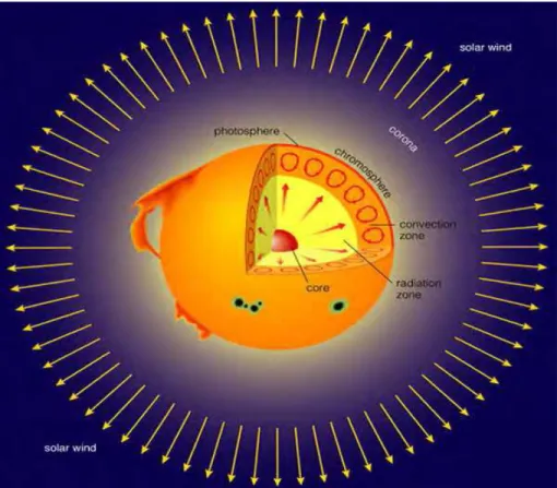
The sun is the source of solar radiation. The nature of the energy radiated by the sun is determined by its structure and its characteristics. The sun is spherical in shape and consists of extremely hot gaseous matter with a diameter of 1.39 × 10⁹ m and it is 1.5 × 10¹¹ m from the earth. A schematic structure of the sun is shown in Fig 2.1. The effective blackbody temperature of the sun is approximately 5777 K whilst the central interior regions have temperatures that vary from 8 × 10⁶ to 40 × 10⁶ K and its density is about 100 times that of water.

Figure 2.1: Structure of the sun (Falayi & Rabiu, Solar radiation models and information for renewable energy applications, 2012).

(36)

23

The sun may be seen as a continuous fusion reactor having its constituent gases as the virtual containing vessel retained by gravitational forces. Energy is produced when hydrogen (i.e. four protons) combine to form helium (i.e. one helium nucleus) which ultimately has a mass less than that of four protons and the difference in mass relates to the produced energy according to Einstein’s formula, 𝐸 = 𝑚𝑐² . The produced energy in the sun’s interior is transferred to its surface where it is radiated into the outer space. This chapter will look in detail how the solar radiation interacts with the atmospheric particles as it makes its way to the earth. The orientation of the sun and the earth will also be discussed, including an introduction of how we get DNI, DHI and GHI.

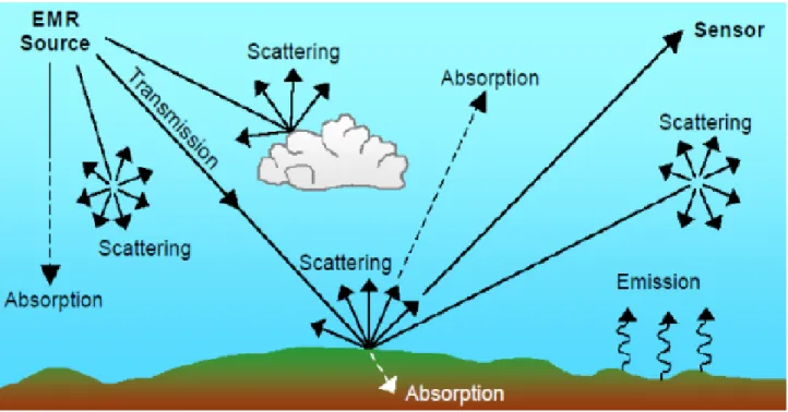
2.1 Interaction of solar radiation with the atmosphere

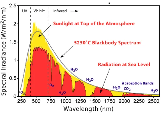
It is a fact that any object with a temperature above absolute zero emits radiation. The sun has a temperature of about 6000 K therefore emits radiation. Radiation emitted by the sun ranges over a wide range of wavelengths. Solar radiation emitted by the sun consists of wavelength that ranges from 300 nm (gamma rays) to 3000 nm (microwaves) and carries electromagnetic energy.

Radiation with shorter wavelength (high frequency) have high energy and that with longer wavelength (low frequency) have lower energy ( Stoffel, et al., 2010). After screening by the layers of the atmosphere, visible light (380 nm < λ < 780 nm) comes out unscattered and reaches the surface in abundance. However, there are some portions of the edges of the visible light that also reach the