Mewomo, A Sectional General Equilibrium Problem with Multiple Output Sets and Joint Fixed Point Problem Submitted to Demonstratio Mathematica. Mewomo, A strong convergence algorithm for multiset equality equilibria and fixed point problems in Banach spaces, submitted to Proceedings of the Edinburgh Mathematical Society.
Research problems and motivation
Research problems
Furthermore, we propose a modified relaxed inertia method for solving monotone variational inclusion problem and common fixed point problem for non-expansive mappings applied to image restorations. In the framework of real Hilbert spaces, we also present a new algorithm for solving the shared common fixed point problem for a class of asymptotic demicontractive mapping.
Motivation
Therefore, it is more difficult to solve SFPs in Banach spaces than in Hilbert spaces. Motivated by this, we extend some of the existing results in these areas to the framework of Banach spaces.
Objectives
Interesting spaces: Hilbert space H is known to have the simplest geometric structure among all Banach spaces. Also, the distance function (also known as the Bregman distance) has been used to facilitate calculations in Banach spaces.
Main Results
Organization of the thesis
Our method uses self-adaptive step size which does not require prior knowledge of the norm operator. The results of numerical experiments demonstrate the comparative advantage of our method over existing methods in the literature.
Some operators in Hilbert spaces
Metric projection
In this subsection, we define the metric projection in a real Hilbert space H and present some of its basic properties with examples. Let C be a non-empty, closed and convex subset of H. Recall that for all x∈H there exists a unique closest point in C denoted by PCx such that.
Some geometric properties of Banach spaces
- Reflexive Banach spaces
- Uniformly convex spaces
- Uniformly smooth spaces
- Duality mappings
- Basic notions of convex analysis
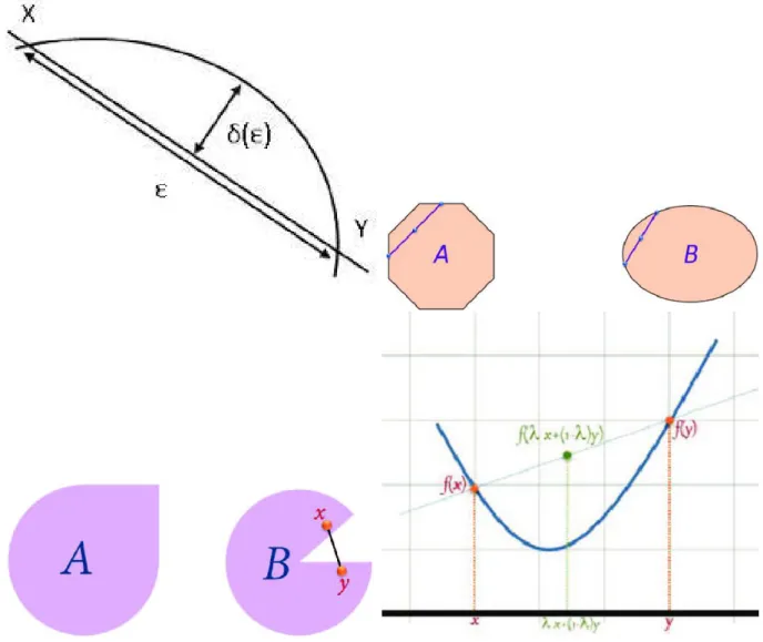
Let p > 1 be a real number, then we say that the Banach space E is p-uniformly convex if there exists a constant c >0 such that δE(ε)≥cεp. In a q-uniformly smooth Banach space E, the generalized duality mapping is injective and satisfies JpE = (JqE∗)−1, where JqE∗ is the generalized duality mapping E∗ (see [10, 66]).
Some important optimization problems
- Minimization problems
- Split convex feasibility problem
- Monotone inclusion problems
- Split monotone variational inclusion problem
- Split hierachical monotone variational inclusion problem
- Variational inequality problems
- Equilibrium and split variational inequality problems
Let C be a non-empty, closed and convex subset of a real Hilbert space H and A:C →H a mapping, the Variational Inequality Problem (VIP) introduced by Lions and Stampacchia [150] is given as defined as follows: Findx∈ C such that. It is well known that the convergence of the gradient projection method requires the cost operator to be strongly monotonic (or conversely strongly monotonic).
Some important lemmas
Then the following statement holds:. i) f is sequentially consistent if and only if it is completely convex on bounded subsets. ii). 231] Let E be a Banach space, s >0a a constant, ρs a measure of the uniform convexity of g, and g : E → R a convex function that is uniformly convex on a bounded subset of E.
Pseudomonotone equilibrium and common fixed point problems
Main result
In this chapter, we present our results on psuedomonotone equilibrium problem and joint fixed point problem of Bregman quasi-nonexpansive mappings in the framework of p-uniformly convex and uniformly smooth Banach spaces. Furthermore, we present our results on partitioned generalized equilibrium problem with multiple output sets and common fixed point problem for an infinite family of multivalued demicontractive mappings in real Hilbert spaces. Next, we prove the strong convergence theorem for the sequence {xn} generated by our proposed algorithm.
The iterative sequence {xn} generated by Algorithm 3.2.2 under Assumption 3.2.1 converges strongly to x∗ ∈Ω, where x∗ =ProjfΩ(u).
Application
Therefore, using Theorem 3.2.8 and Lemma 3.2.9, we obtain the following result for approximating the joint solution of the pseudo-monotone variational inequality problem and the joint fixed point problem for a finite family of Bregman quasiexpansive mappings to a p-uniformly convex real Banach space, which is also uniformly smooth. Let E be a p-uniformly convex real Banach space that is also uniformly smooth, and let C be a nonempty, closed and convex subset of E .
Numerical experiments
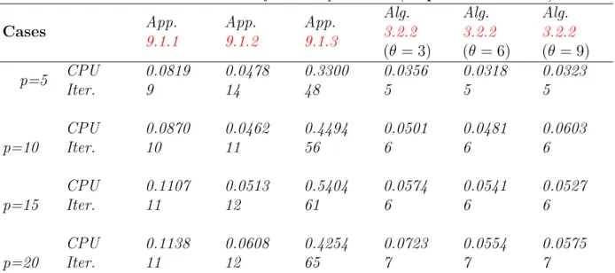
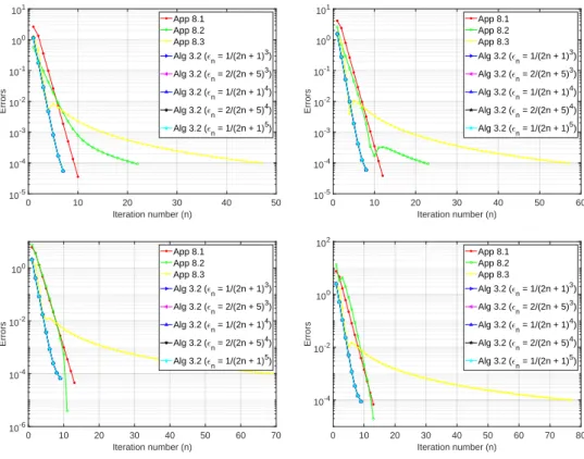
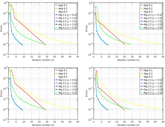
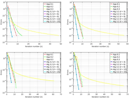
In this experiment, we check the behavior of our method by fixing the other parameters and changing θ in Example 3.2.12. In this experiment, we check the behavior of our method by fixing the other parameters and changing ρ in Example 3.2.14. In Experiment 3.2.15, we investigate the sensitivity of θ for each case of p to know whether the choices of θ affect the performance of our method.
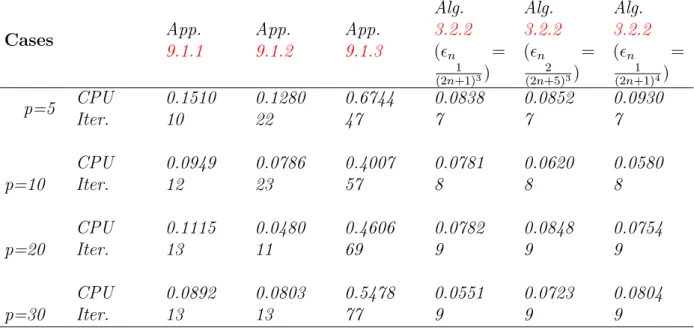
In Experiment 3.2.16, we examine the sensitivity of ϵn for each case of p in order to know whether the choices of ϵn affect the performance of our method.
Split generalized equilibrium problem with multiple output sets
Main result
In this section, we present a modified viscosity-type algorithm for approximating a common element of the solution set of the generalized partitioned equilibrium problem with multiple output sets and the common fixed point problem for an infinite family of many-valued demicontractive mappings in real Hilbert spaces. . Fori= 1,2, .., N, let Cibe nonempty closed convex subsets of Hilbert spacesHi and letAi :H→Hibe bounded linear operators. This follows from the limit of the operators Ai, the nonexpansiveness of the mappings Tr(Fi i,ϕi) and the limit of the sequence {xnk} that.
N in Theorem 3.3.8, we have the following consequent result for approximating a general solution of the set solution of split equilibrium problem with multiple output sets and the common fixed point problem for an infinite family of multivalued demiconstructive mappings in real Hilbert spaces .
Application
Consequently, Corollary 3.3.9 can be used to approximate the common solution of SVIPMOS (3.86) and the common fixed point problem for an infinite family of multivalued demicontractive mappings Sj : H → CB(H), j ∈N in real Hilbert spaces, where the solution quantity given with Γ :=T∞.
Numerical examples
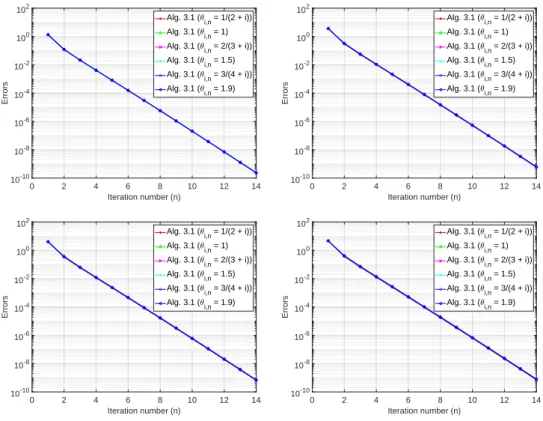
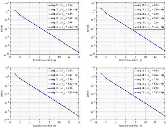
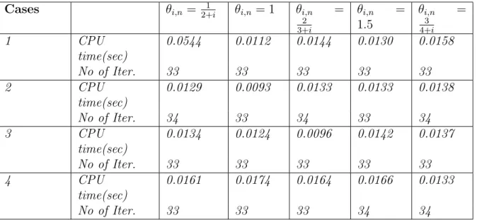
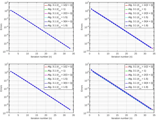
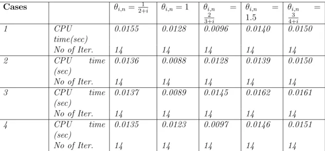
In this experiment, we check the behavior of our method by fixing the other parameters and varying θi,n. We use Algorithm 3.3.5 for the experiment and report the numerical results in Table 3.2.11 and Figure 3.4. In this experiment, we check the behavior of our method by fixing the other parameters and varying ϕi,n. We do this to check the effects of the parameter ϕi,n on our method.
We use Algorithm 3.3.5 for the experiment and report the numerical results in Table 3.2.12 and Figure 3.5.
Non-Lipschitz split monotone variational inclusion problem with fixed points
Main result
In this chapter, we present our results of a relaxed double-inertial Tseng extragradient method with self-adaptive step sizes for solving the split monotone variational inclusion problem (SMVIP) involving non-Lipschitz operators and the fixed point problem of strict pseudocontractive mappings. Furthermore, since T is a bounded linear operator, we have T wnj ⇀ Tx.ˆ From (4.40) and the continuity of D, it follows that. Further, since I−Sα is demichlorinated to zero, we have by Lemma 2.5.13 and the fact that ∥Sαvnk−vnk∥ →0.
Moreover, since {xnk} is bounded, there exists a subsequence {xnkj} of {xnk} that converges weakly to x† ∈H1 and.
Applications
With Lemma 4.1.11 in mind and setting D = 0, A = 0 in Theorem 4.1.10, we obtain the following relaxed double inertia method from Algorithm 4.1.2 to approximate the joint solution of split equilibrium problem (4.76) and (4.77) ) and fixed point problem with strict pseudocontractive mappings in the framework of real Hilbert spaces. Suppose that Assumption 4.1.1 holds, then the iterative sequence {xn} generated by Algorithm 4.1.12 converges strongly to an element of Υ. It is a well-known fact that the gradients ∇f1 and ∇f2 off1 and f2 respectively are monotonic and continuous (see [26]).
Suppose assumption 4.1.1 holds, then the iterative sequence {xn} generated by algorithm 4.1.14 converges strongly to an element of Υ.
Numerical example
Generalized split feasibility problems
Main result
Application to image restoration problems
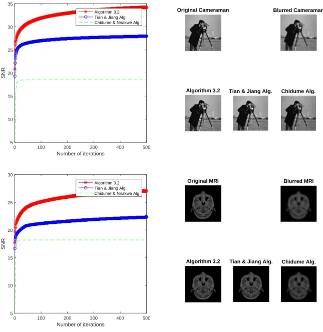
In addition, we use Gaussian blur of size 9 × 9 and standard deviation σ = 4 to generate a blurred and noisy image (observed image). We also measure the quality of the reconstructed image using the signal-to-noise ratio, defined as Then, the results are shown in Table 1, which shows the CPU time and SNR values for each algorithm, and Figure 1, which shows the original, blurred, and restored images.
The two major advantages of our Algorithm over the other two algorithms are the higher SNR value and lower CPU time for generating the restored images.
Numerical experiments
We now summarize this section by focusing on some observations from the numerical results. During numerical calculations, we noticed that regardless of the choice of parameters γ1, λ1 > 0, µ, η ∈ (0,1) and α ≥ 3, the number of iterations does not change and there is no significant difference in processor time. . Through experiments, we clearly see that Algorithm 4.2.11 is better than Algorithm 4.2.3 and Algorithm 4.2.9 both in terms of CPU time and number of iterations.
We can also see from the cases that regardless of the choices of the relaxation step size, our proposed methods converge more than twice as fast as the other methods.
Introduction
Variational inequality and fixed point problems
Main result
By the definition of subgradient, we note that C ⊂Cn. b) The step size {λn} given by (5.2) is generated at each iteration by a few simple calculations. Since yn =PCn(wn−λnAwn) and p ∈Cn, then by characterization we have PCn. Since wnj ⇀x,ˆ by the assumption of the lemma it follows that ynj ⇀xˆasj →+∞. Using the Cauchy-Schwartz inequality, we have
By the limits of {xnk}, there exists a subsequence {xnkj} of {xnk} such that xnkj ⇀ x† and.
Applications
Numerical example
It can be easily verified that C is a non-empty closed convex subset of H. The operator A:H →H is given by. It is easy to see that A is monotonic and Lipschitz is continuous on H with the Lipschitz constant L = 2.
Two-level variational inequality and fixed point problems involving pseu-
Main result
Let {xn} sequence be generated by Algorithm5.3.1 under Assumptions S. Suppose there exists a subsequence {xnb} of {xn} that converges weakly to x¯ ∈ H and lim. Proof of Claim: Let {xnq}q≥0 be a sequence of {xn}n≥0 such that lim sup. which converges weakly to ¯x in H. For convenience, and WLOG, we will represent {xnqb}b≥0 by {xnb}b≥0. This completes the proof for the first case. 5.89) Furthermore, following the arguments used in Case 1, we obtain that
The result extends to the solution of variational inequality problem of monotone operators since every pseudo-monotone operator is monotone.
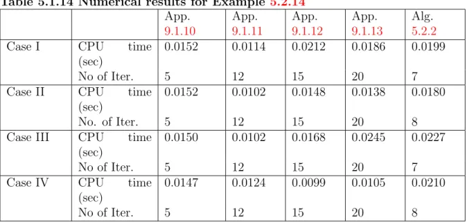
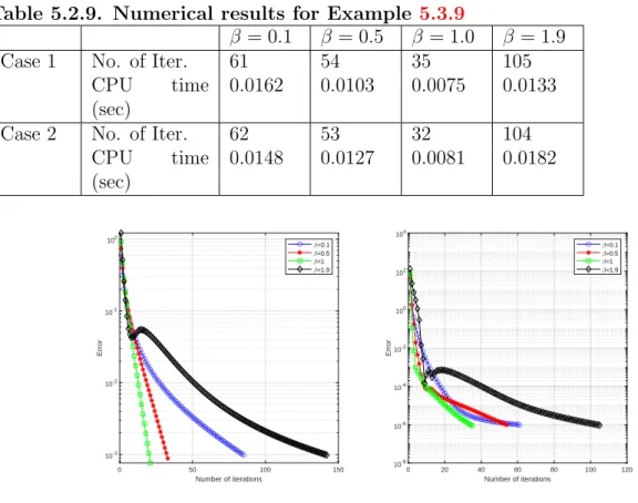
Numerical example
The exact solution to the problem is x∗(t) = 0. Since the solution is known, we use the sequence E(xn) =∥xn−x∗∥2 for every n ≥0 to test the numerical behavior of our algorithm. to illustrate .
An inertial extrapolation method for solving
Main result
Computeyn:=un−ηn(un−zn), where ηn:=αmn andmn is the smallest non-negative. a) Assumption b) requires the operator. A is pseudomonotonous and uniformly continuous, which is much more, a weaker assumption than the monotonicity and Lipschitz continuity assumptions used in, as well as the inverse strongly monotonic assumptions used in other papers for solving split-variation problems— inequality (see e.g. Thus, our method is applicable to a much more general class of Pseudomomonotonic and uniformly continuous operators.
Therefore, our method is computationally less expensive than other methods in the literature for solving split variation inequality problems.
Numerical example
Split common fixed point problem of asymptotically demicontractive map-
Main result
Numerical examples
Split minimization problem with multiple output sets and common fixed
Main result
Applications
Numerical Examples
On split equality equilibrium, monotone variational inclusion and fixed
Main results
Application
Multiple set split equality equilibrium and fixed point problems
Main result
Convergence analysis
Application
Numerical example
Contributions to knowledge
Future research
Appendix
Appendix
Appendix
Appendix
Appendix
This is expected because Algorithm 4.2.11 does not require any estimate of A and the step size λn in Algorithm 4.2.11 does not involve any form of "inner loop" during execution that is required in Algorithm 4.2.3 and Algorithm 4.2.9 . The set C is defined by. where c:H →R fulfills the following conditions:. a) c : H → R is a continuously differentiable convex function such that c′(.) is M-Lipschitz continuous;. Thus, {λn} is easy to implement and does not depend on the Lipschitz constant of the cost operator.
So there exists p ∈Ω such that p=PΩ(I−D+γf)(p). Since p∈Ω, then we have thatVp=p. Next, we get from the definition of wn. Then the sequence {xn} strongly converges to a point p ∈ Ω, where p = PΩ(I − D+γf)p is a solution of the variational inequality. Then the sequence {xn} strongly converges to a point p ∈ Ω, where p=PΩ(I−D+γf)p is a solution of the variational inequality.