Models for the risk factors (covariates) of HIV incidence are considered in the last chapter, except for one. KEYWORDS: HIV incidence; Cohort studies; Cross-sectional surveys; Maximum likelihood; previous appearance; appearance density; sensitivity and specificity; risk factors.
Introduction
In particular, one of the major public health goals is to reduce the incidence of HIV (Guy et al., 2009). This method is known as the serological testing algorithm for recent HIV seroconversion (STARHS), (Janssen et al., 1998).
Data Description
- Introduction
- Laboratory Testing
- The Data
- Preliminary analysis
- Limitations of the Data
We performed a chi-square test for the association between outcome status and each of the above variables. One of the main limitations of this dataset was that, except age and gender, all other variables contained a lot of missing information.

Thesis Objective
For this reason, we used age and gender only to illustrate the proposed methods and to address the question of the dependence of incidence on covariates.
Thesis Outline
The effectiveness of the proposed method is evaluated through a simulation study and its application is demonstrated. We use data from the 2008 Botswana AIDS Impact Survey (BAIS) III to illustrate the application of the proposed method in Section 2.5.
Models and the likelihood function
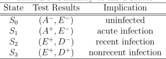
Review of the Four-State Balasubramanian-Lagakos (BL) Model 16
Finally, S3 represents the "non-recent infection" state in which HIV antibodies can be detected by a less sensitive test (and sensitive test). Finally, S3 represents the "non-recent infection" state in which HIV antibodies can be detected by a less sensitive test and sensitive test.
The extended model allowing for past prevalence
Incorporating false recent rate into the extended model
The model we presented in section 2.3 does not take into account individuals who remain negative indefinitely on a less sensitive test. End state 4 represents subjects that can be detected by a sensitive assay but will remain permanently unreactive to a less sensitive assay.
The likelihood function and parameter estimation
Since the estimator we introduced in Section 2.3 is also a maximum likelihood estimator, to include the false posterior rate, we extend the approach of Wang and Lagakos (2009). According to this model, state 1 represents the “pre-seroconversion” state that corresponds to the period in which an individual is either infected but not yet seroconverted or is uninfected.
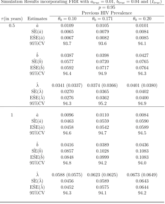
Simulation Study
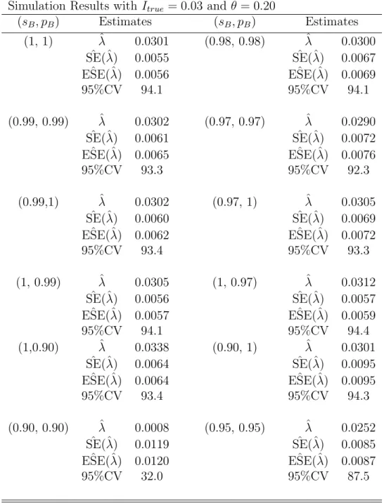
In general, ˆSE(ˆλ) and ESE(ˆˆ λ), the estimated standard errors and the corresponding empirical estimates, are very close to each other for all different time points for both models. The estimated standard errors are closer to the corresponding empirical estimates in both cases of the latter false proportions, 5% and 2%, respectively.
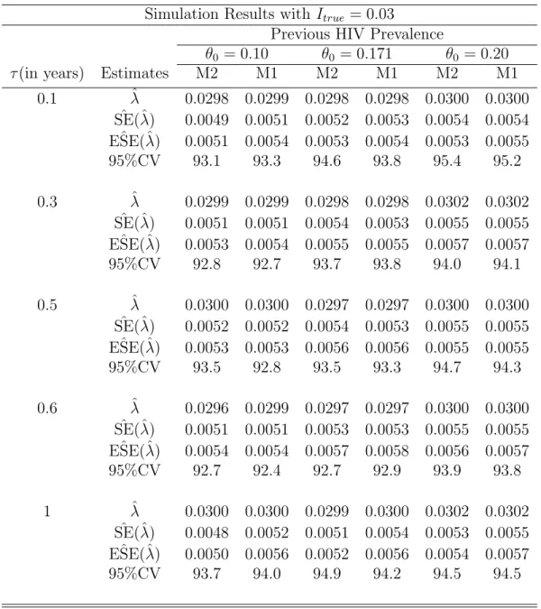
Illustration of the proposed model using BAIS III data set
However, the proposed method does not take into account the uncertainty of the fake latest rate and the average window period. Although the uncertainty in the false recent rate and the average window period affects estimators of incidence, we note that for comparison between the two methods, the uncertainty in the two estimators will not affect the conclusions.
Introduction
Adjustment procedures to deal with these misclassifications were first proposed by Parekh et al. 2006) adjustment method uses sensitivity (proportion of recent samples that are positive, i.e. below the normalized optical density threshold) in the mean window period (µ) and short-term and long-term specificity (proportion of long-term samples that test negative, i.e. above normalized optical density threshold). Overall, Hargrove et al. 2008) adaptation is a simplified version of McDougal et al. 2006), assuming that sensitivity and short-term specificity are the same. In particular, Hargrove et al. 2008) depends mainly on the spurious recency rate and the mean period of the window.
This could be an expensive exercise, as reported by Janssen et al. 1998), who later proposed a simple three-state model.
Preliminary Concepts
In the remaining sections, we proceed as follows: the proposed method is introduced in Section 3.3. We define specificity (pB) for the BED test as the probability that the BED test is negative given that the subject is in state S1 or S2.
Incorporating Imperfect Sensitivity and Specificity
Simulation
Application to BAIS III data set
Introduction
Results
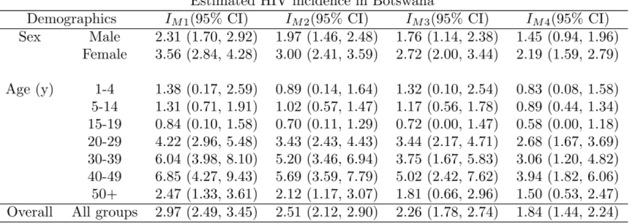
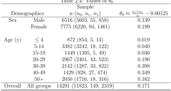
The HIV prevalence rate is higher for the middle age groups (20-49 years) in accordance with what is reported in the literature, for example in CSO (2008).
Discussion
More research is needed to investigate the effect of ART use on HIV incidence estimation. But if a biased mean period estimate is used, all estimates of HIV incidence will also be biased. In this paper, we relax this assumption and derive the maximum likelihood estimator (MLE) of HIV incidence.
In particular, we derive the MLE of HIV incidence if the incidence density is assumed to be linear.
A review of the constant incidence density model
In addition, let f(t), F(t) and λ(t) denote the density function (incidence density), the cumulative distribution function and the hazard function for infection at time t. Let L2 denote the residence or residence time in S2 with the corresponding cumulative distribution denoted by G2(·) as in Balasubramanian and Lagakos (2010) and the corresponding probability density function given by g2(·). However, Balasubramanian and Lagakos (2010) proposed a more general framework that combines information from all three states with a likelihood approach using a multinomial distribution and then derives a maximum likelihood estimate of HIV incidence along with corresponding estimates of their standard. mistakes.
This paper puts forward the idea of relaxing this assumption and considering other forms of f(t) over [t−L∗2, t].
Linear Incidence Density Form
Inference
To construct approximate confidence intervals for (a, b, θ, or λ), the standard errors for their MLEs or their component functions can be obtained from the Hessian matrix H of the log-likelihood function. In the proposed model, we assume that all subjects are tested with two diagnostic tests, which consist of a standard ELISA test and a BED test. If we replace 'a' and 'b' by their respective MLEs given in equation (4.3.5) and equation (4.3.6) respectively in equation (4.3.8), it follows that the approximate variance ˆa, variance ˆb and covariance between ˆa and ˆb are:.
Incorporation of the false recent rate
HIV-infected subjects may remain nonreactive to the less sensitive assay indefinitely after the seroconversion period, leading to overestimation of the estimated HIV incidence rate as discussed by (Wang and Lagakos, 2009; McWalter and Welte, 2010; Brookmeyer, 2010b; Hargrove et al., 2008; Novitsky et al., 2009; Karita et al., 2007). Let denote the proportion of subjects who will become reactive at some point after seroconversion as in Wang and Lagakos (2009). Then the false recent rate will be q = 1−p, which indicates the proportion of subjects who remain negative on the less sensitive assay indefinitely.
Therefore, the MLE of HIV incidence at time t, ˆλ(t), which is now a function of pores, will be equal to q= 1−p.
Testing For b=0
The significance level represents the chance that the reduced model (when b=0) is rejected when it is actually the correct model for the data.
Simulation Study
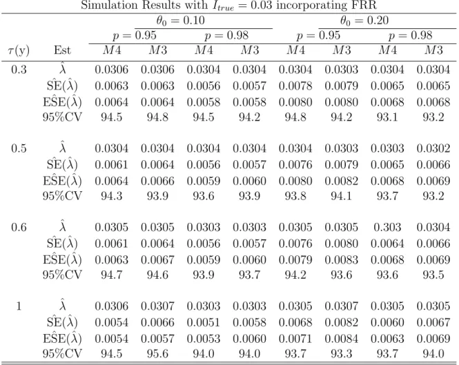
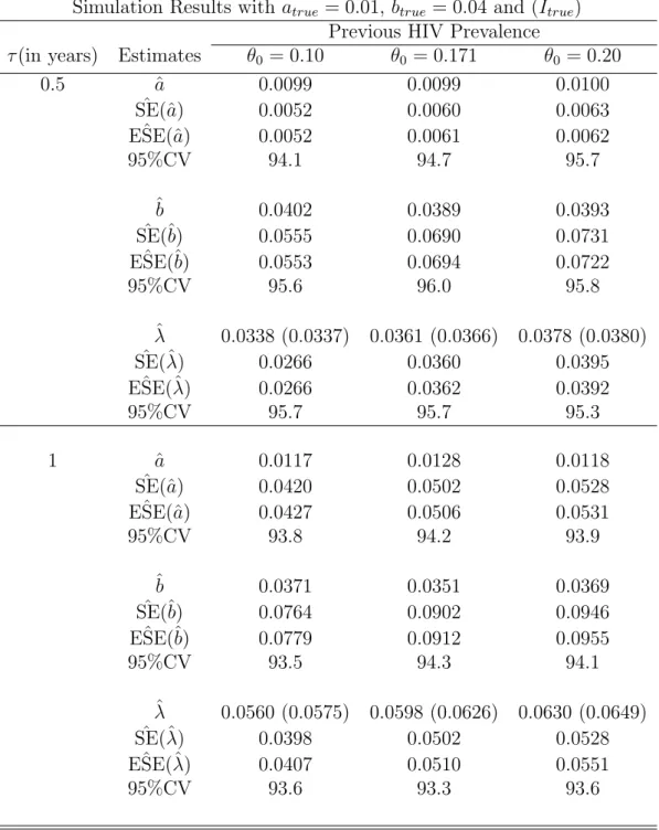
We also obtain the empirical estimates of the variance from the 1000 simulated point estimates of incidence. The standard errors of the unadjusted estimators are consistently lower than those of the adjusted estimators. It is also reassuring to note that the estimated standard errors and the empirical estimates are closer to each other for all the estimates.
The estimated standard errors decrease as the proportion of non-progressors (false recent rate) decreases.
Application to BAIS III data set
The last row of the table also gives the total score for each parameter estimate. That is, we tested whether the assumption of a linear incidence density was reasonable for these data in these settings as opposed to the assumption of a constant incidence density (the prior prevalence is assumed to be known). The results show that for p = 1 and p = 0.98 we reject the assumption of constant incidence density and conclude that the assumption of linear incidence is reasonable in these settings (p values < 0.01).
This is an indication that the force of the infection or the intensity of the disease is more pronounced in the younger age groups and reaches a maximum in the age group 40 -49 and less pronounced in the older age groups after 50 years and above.
Discussion
However, for some reasons, known or unknown, a proportion of samples that test positive with a standard antibody test may not be tested with a less sensitive test, resulting in missing data. However, for some reasons, known or unknown, a proportion of samples that tested positive with the sensitive antibody test are not tested with the less sensitive test, resulting in missing data. Another way of dealing with missing data was presented by Chu and Cole (2006) using the maximum likelihood method under the assumption of missing at random (MAR), as described by Little and Rubin (2002).
In Section 5.2, we describe the maximum likelihood method for imputing missing data to MAR.
The extended model incorporating missing data
Ad hoc methods for including missing data assume that the missing data is missing completely at random (MCAR). Finally, state 3, designated S3, represents the “non-recent infection” state in which HIV antibodies are detectable by a less sensitive test (and sensitive test). Using similar arguments as in Balasubramanian and Lagakos (2010), it can be shown that the prevalence probabilities for the 3-states at time t are equal.
Note that nm is the number of missing samples that tested positive on the sensitive test and they are a fraction of prevalent cases (new and long-standing cases), hence the expression nmlogθ, where θ is the HIV prevalence at time t.
Application to BAIS III data set
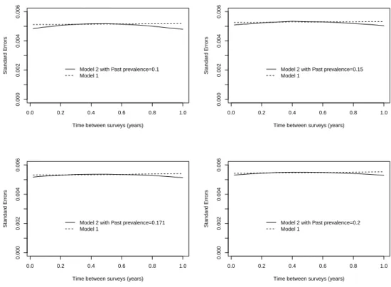
In addition, Table 5.1 also presents the estimated HIV prevalence together with the associated 95% confidence intervals (95% CI). We note that Model 1 produces values of the estimated incidence that are larger than those of Model 2. The difference in the estimated incidence in the two models is not large because the number of missing instances is not too large.
However, if we consider the fact that only 67% of the targeted individuals provided the blood sample for HIV testing, the impact of missing information on the estimated prevalence could be severe.

Discussion
Understanding the risk factors for HIV incidence is essential for the allocation of resources and proper implementation of risk reduction programs and other intervention strategies. In this paper, we follow the procedure similar to that developed by Balasubramanian and Lagakos (2010) to examine the risk factors associated with HIV prevalence through a multiple logistic regression model. Understanding the risk factors for HIV incidence is essential for the allocation of resources and proper implementation of risk reduction programs and other intervention measures.
This paper follows the procedure developed by Balasubramanian and Lagakos (2010) to investigate risk factors associated with HIV incidence through a multiple logistic regression model.
The incidence rate ratio
Incorporating Covariate Dependence
Logistic Regression Method
The logistic regression model assumes that the logarithm of the probabilities of the outcome is a linear function of the predictors. We also use the logistic regression model proposed by Balasubramanian and Lagakos (2010) and extend the idea of Magder and Hughes (1997) to incorporate the uncertainty of the interest rate outcome. The developed methods use the statistical framework developed by Balasubramanian and Lagakos (2010) to derive probability estimators of incidence.
However, as mentioned earlier in most chapters, we still have challenges in estimating HIV incidence rates. A simulation study to evaluate the performance of the new incidence estimator adjusting for sensitivity and specificity. A simulation study to evaluate the performance of the new incidence estimator under the linear incidence density function.