The potential of hyperspectral remote sensing in determining water turbidity as a water quality indicator
Dumisani Solly Mashele 203513086
A thesis submitted to the School of Agricultural, Earth and Environmental Sciences, at the University of KwaZulu-Natal, in partial fulfillment of the academic requirements for the
degree of Master of Environment and Development (MEnvDev), Land Information Management
March 2013 Pietermaritzburg
South Africa
i DECLARATION
This research work was undertaken in partial fulfillment of a Master of Environment and Development (MEnvDev), Land Information Management offered through the School of Agricultural, Earth and Environmental Sciences. I would like to declare that the research work reported in this thesis has never been submitted in any form for any degree or diploma to any tertiary institution. It, therefore, represents my original work .Where use has been made of the work of other authors or organizations it is duly acknowledged within the text and references list.
Dumisani Solly Mashele (203513086)
Signed: __________________________________Date:_________________
As the candidate’s supervisor, I certify the above statement and have approved this thesis for submission.
Dr John Odhiambo Odindi
Signed: __________________________________Date:_________________
ii PLAGIARISM DECLARATION
I, Dumisani Solly Mashele, declare that:
1. The research reported in this thesis, except where otherwise indicated is my original work.
2. This dissertation has not been submitted for any degree or examination at any other university.
3. This dissertation does not contain other persons’ data, pictures, graphs, or other information, unless specifically acknowledged as being sourced from other persons.
4. This dissertation does not contain other persons’ writing, unless specifically acknowledged as being sourced from other researchers. Where other written sources have been quoted, then:
a. Their words have been re-written, but the general information attributed to them has been referenced.
b. Where their exact words have been used, then their writing has been placed in italics and inside quotation marks, and referenced.
5. This dissertation does not contain text, graphics, or tables copied and pasted from the Internet, unless specifically acknowledged and the source being detailed in the thesis and in the References Section.
Signed: ________________________________
iii
TABLE OF CONTENTS
DECLARATION... i
PLAGIARISM DECLARATION... ii
TABLE OF CONTENTS ... iii
LIST OF FIGURES ... v
LIST OF TABLES ... vi
ABSTRACT ... vii
ACKNOWLEDGEMENTS ... viii
CHAPTER 1: INTRODUCTION ... 1
1.1 Introduction ... 1
1.1.1 Turbidity and water quality ... 2
1.2 Aim of the study... 3
1.3 Research objectives ... 3
1.4 Structure of thesis ... 4
2.1 Water resources ... 5
2.1.1 Water resources: a general outlook ... 5
2.1.2 Water resources in South Africa ... 5
2.2 Water quality ... 6
2.2.1 Physical attributes ... 6
2.2.2 Chemical attributes ... 6
2.2.3 Biological attributes... 7
2.3 Water quality in South Africa ... 7
2.3.1 A general overview ... 7
2.3.2 Causes of water pollution ... 7
2.4 Water turbidity ... 8
2.5 Turbidity measurement ... 9
2.6 The application of remote sensing in water quality ... 10
2.6.1 Estimating turbidity ... 13
2.7 Methods of estimating water quality constituents ... 15
2.7.1 Analytical ... 15
2.7.2 Empirical... 15
iv
2.8 Algorithm development ... 16
2.9 Summary ... 17
CHAPTER 3: RESEARCH METHODOLOGY ... 18
3.1 Introduction ... 18
3.2 Data acquisition and methods ... 18
3.2.1 Study area ... 18
3.2.2 Soil samples ... 19
3.2.3 Spectral measurements of turbid solutions ... 20
3.2.4 Laboratory turbidity measurements ... 21
3.3 Processing ... 22
3.3.1 Initial spectra processing ... 22
3.3.2 Estimating turbidity ... 22
3.3.3 Model validation ... 24
3.4 Summary ... 24
CHAPTER 4: RESULTS ... 25
4.2 Soil properties and reflectance ... 25
4.3 Turbidity ... 26
4.4 Spectral characteristics of different turbidity levels ... 28
4.5 Optimal bands ... 30
4.5.1 Visible region ... 30
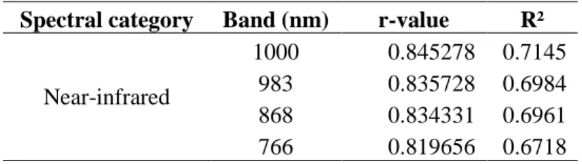
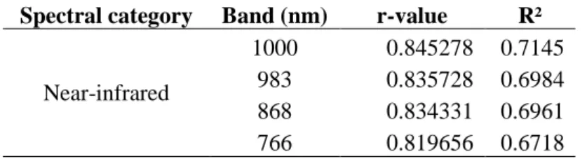
4.4.2 Near-infrared region ... 32
4.4.3 Spectral indices ... 34
CHAPTER 5: DISCUSSION AND CONCLUSION ... 38
5.1 Introduction ... 38
5.2 Conclusion ... 40
REFERENCES ... 41
APPENDIX A: SPECTRAL DATA ... 49
APPENDIX B: SOIL ATTRIBUTES ... 56
APPENDIX C: PLOT OF R2 AND P VALUES FOR ALL BANDS ... 56
v LIST OF FIGURES
Figure 1: Spectral responses of common materials ... 11
Figure 2: Change in reflectance against turbidity ... 12
Figure 3: Sources of electromagnetic radiation ... 13
Figure 4: The distribution of sample sites in the study area ... 19
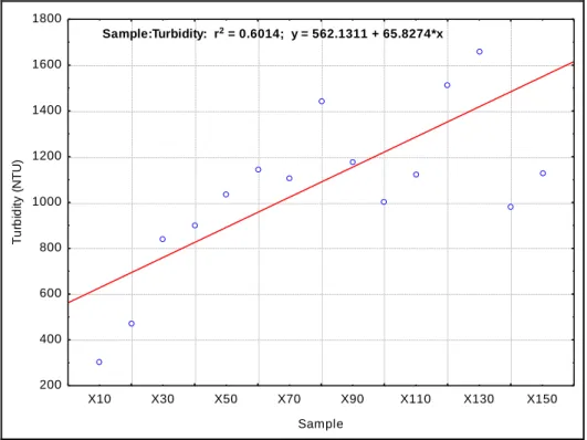
Figure 5: Laboratory based turbidity data distribution ... 27
Figure 6: Average laboratory based turbidity measurements against amount of soil in solution. ... 28
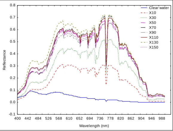
Figure 7: A general spectral reflectance characteristic of turbid and clear water with absorption bands ... 29
Figure 8: Spectral reflectance of solutions with varied amounts of soil ... 30
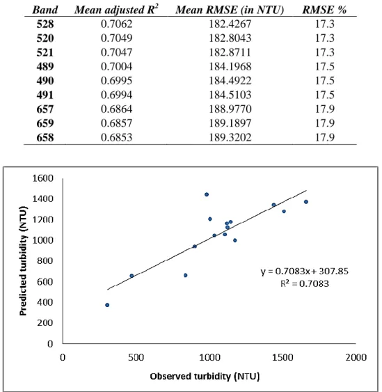
Figure 9: Regression model of observed and predicted turbidity at 528nm ... 31
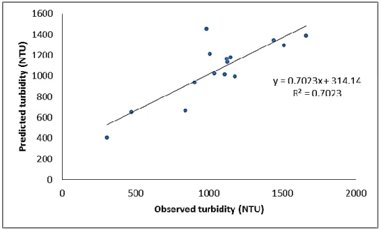
Figure 10: Regression model of observed and predicted turbidity at 489nm ... 32
Figure 11: Regression model of observed and predicted turbidity at 657nm ... 32
Figure 12: Regression model of observed and predicted turbidity at 1000nm ... 33
Figure 13: Regression model of observed and predicted turbidity at 983nm ... 33
Figure 14: Regression model of observed and predicted turbidity at 625/440 ... 36
Figure 15: Regression model of observed and predicted turbidity at (770-1000) / (770+1000) ... 36
vi LIST OF TABLES
Table 1: Formulae for spectral indices ... 23
Table 2: Physical and chemical properties of soil samples used ... 26
Table 3: Descriptive statistics of measured turbidity (in NTU) ... 27
Table 4: Visible region bands ... 30
Table 5: LOOCV results of visible bands ... 31
Table 6: Near-infrared region optimal bands ... 33
Table 7: LOOCV results of near-infrared bands ... 34
Table 8: Tested spectral indices ranked according to R2 ... 35
Table 9: LOOCV results of selected spectral indices ... 37
vii ABSTRACT
Globally, water turbidity remains a crucial parameter in determining water quality. South Africa is largely regarded as arid and is often characterised by limited but high intensity rainfall. This characteristic renders most of the country’s water bodies turbid. Consequently, the use of turbidity as a measure of water quality is of great relevance in a South African context. Generally, turbidity alters biological and ecological characteristics of water bodies by inducing changes in among others temperature, oxygen levels and light penetration. These changes may affect aquatic life, ecosystem functioning and available water for industrial and domestic use. Siltation, a direct function of turbidity also impacts on the physical storage of dams and shortens their useful life. To date, determination of water turbidity relies on the tradition laboratory based methods that are often time consuming, expensive and labour intensive. This has increased the need for more cost effective means of determining water turbidity.
In the recent past, the use of remote sensing techniques has emerged as a viable option in water quality assessment. Hyperspectral remote sensing characterizes numerous contiguous narrow bands that have great potential in water turbidity measurement. This study explored the applicability of hyperspectral data in water turbidity detection. It explored the visible and near-infrared region to select the optimal bands and indices for turbidity measurement. Using the Analytical Spectral Device (ASD) field spectroradiometer and a 2100Q portable turbidimeter, spectral reflectance and laboratory based turbidity measurements were taken from prepared turbid solutions of predetermined concentrations (i.e. 10g/l to 150g/l), respectively. The Pearson’s coefficient of correlation and R2 values were employed to select optimal spectral bands and indices. The findings showed a positive linear relationship between reflectance, the amount of soil in water and turbidity values. The strongest relationships came from bands 528, 489, 657, 1000 and 983, reporting adjusted R2 values of 0.7062, 0.7004, 0.6864, 0.7120 and 0.6961, respectively. The highest coefficient came from band 1000nm. The strongest indices were 625/440 and (770-1000)/(770+1000), with adjusted R2 values of 0.6822 and 0.6973 respectively. The use of hyperspectral data in turbidity detection is ideal for optimal band interrogation. Although good results were generated from this study, further investigations are needed in the near-infrared region.
viii ACKNOWLEDGEMENTS
Firstly, I wish to express my deepest gratitude to the Almighty God for the grace He has extended to me by His son and my Lord Jesus Christ. You are the sum total of all my endeavours.
My sincere appreciation goes to my supervisor Dr JO Odindi for his motivation, guidance, patience and support throughout the research. Without him this work would have not been successful.
I thank Dr E Adam for his excellent assistance and advices on data collection, preparation and analysis. My knowledge and technical skills in remote sensing have improved immensely because of you.
To my colleague and brother, Mr C Adjorlolo, thank you for the ideas, academic interrogations and honest feedback to my seemingly never-ending questions. You helped sharpen my understanding in research.
I extend my gratitude to my boss Mrs. FJ Mitchell for her continued understanding and support and also to the Department of Agriculture and Environmental Affairs for helping with the soil and water analyses.
To my parents (Mr PJ and Mrs. M Mashele), brothers (Sifiso and Luyanda) and sisters (Olgar, Siphiwe and Thobile), thank you for always believing in me. Your love and support have continued to propel me forward to succeed.
Finally, I want to thank my beautiful wife, Portia Nombuso Ngcobo (now a Mashele), for being a true friend, my personal chief advisor, my strength and number one supporter. I love you always.
1 CHAPTER 1: INTRODUCTION
1.1 Introduction
Water constitutes three quarters of the Earth’s surface (Plaza et al., 2004). Of that amount only 2.5% is fresh-water and exists as permanent snow cover and glaciers, groundwater, soil, swamps, lakes and rivers (Shiklomanov, 1998). Due to a rise in population, industrial development and expansion of irrigation agriculture, water use has increased six-fold over a period of 70 years (Bernstein, Undated). The quality of available water has also declined.
According to Bernstein (Undated), about 1.1 billion people are deprived of clean water. Poor water quality is reported as one of the leading causes of death in poor communities (Venter, 2002, WRC, 1998).
Over 65% of the African continent is classified as arid or semi-arid (Clark, 2010). Clark (2010) further notes that the continent accounts for only 9% of global renewable freshwater resources. Environmental related threats like forest and biodiversity loss, land degradation and urbanization caused by ever increasing population have further led to a decline in water quality and quantity (Clark, 2010, Eva et al., 2006). Like other African countries, South Africa is characterised by perennial water stress and scarcity (Eva et al., 2006).
With an average total annual rainfall of 450mm compared to the world’s 860mm, South Africa is regarded as a semi-arid country (CSIR, 2010). Over 90% of her mean annual rainfall is lost to the atmosphere through evaporation (Whitmore, 1971 as cited by Schulze, 1995) and only about 8.5% of the available water translates to runoff (Backeberg et al., 1996). A large portion of the available water is often allocated for use, leaving virtually no surplus water. Furthermore, the country’s fast growing population, changing standard of living and recent government drive to establish “decent” human settlements has further increased pressure on the existing water resources (Ashton, 2007, CSIR, 2010, Fatoki et al., 2001). Increased volumes for domestic, industrial and agricultural, mining and power generation have combined with land use associated problems like soil erosion to degrade the quality of the country’s water resources (CSIR, 2010, Du Plessis, 2006).
2 1.1.1 Turbidity and water quality
Turbidity is an important water quality indicator that measures the relative clarity of water (Lambrou et al., 2010). It basically amounts from suspended silt and clay particles, algae, organic matter and microscopic organisms in water bodies affect their color and brightness (Kwoh et al., Undated, Ramollo, 2008). Generally, turbidity interferes with a water body’s light transmission which affects submerged aquatic plant’s primary productivity (Hart, 1999, Norsaliza and Hasmadi, 2010a, Norsaliza and Hasmadi, 2010b, Ramollo, 2008).
Furthermore, turbidity reduces the amount of oxygen in water which may cause plant death, organic matter decay and induce production of carbonic acid (Hart, 1999). The subsequent suppressed production in aquatic plants reduces food availability, which in turn affects biota distribution and habitat selection (Dörgeloh, 1995, Hart, 1999). Because suspended particles absorb more sunlight they increase water temperature, leading to further depletion of dissolved oxygen as warm water holds less oxygen than cool water (Ramollo, 2008). These conditions lead to aesthetically undesirable and un-inhabitable water bodies devoid of life.
South Africa’s water resources are particularly affected by turbidity. Almost all of the country’s reservoirs are turbid (Dörgeloh, 1995, Dörgeloh et al., 1993). The country’s reserviors turbidity levels are largely attributed to arid conditions associated with high intensity rainfalls on areas with limited vegetation and consequent soil erosion (Hart, 1999).
Other turbidity causative factors include domestic and industrial effluents and agrochemicals from agriculture (Ashton, 2007). Ultimately most of the water from these sources is drained into rivers.
Turbidity does not only have environmental and ecological consequences in river systems but also pose an economic threat, through facilitating reservoir siltation. Such makes its measurement and monitoring a valuable exercise. Traditional methods used to determine turbidity like in situ measurements and laboratory analyses play a significant role in monitoring water quality. However, these techniques are time-consuming, expensive and labour intensive (He et al., 2008, Liu et al., 2003, Shafique et al., 2003, Su et al., 2008b, Yang et al., 2000, Yang and Jin, 2010). Generally, the use of these techniques is often required for wider temporal and spatial scale, which remains a challenge (Bierman et al., 2011).
Turbidity analysis using remote sensing techniques offers a great opportunity in water quality management. These techniques permit for more efficient data collection and analyses, which
3 offer opportunities to identify other implicit relationships (Koponen, 2006, Senay et al., 2001). Recent improvement in sensor spatial and spectral resolutions and point based spectroscopy has facilitated the investigation of various aspects of water quality. A number of studies have successfully explored remote sensing application techniques in water quality.
These studies have investigated the water quality parameters that include among others pH, salinity, chlorophyll a, total phosphorus and temperature, total suspended sediments and turbidity (Akbar et al., Undated, He et al., 2008, Norsaliza and Hasmadi, 2010a, Norsaliza and Hasmadi, 2010b, Pavelsky and Smith, 2009, Su et al., 2008a, Wu et al., 2007, Zhengjun et al., 2008). What is limiting about most of these studies is that they used broad band spectral categorization of reflected and emitted energy, covering the visible to near-infrared regions (Govender et al., 2007). The use of hyperspectral remote sensing using a spectrometer permits several hundreds of spectral bands to be collected at one time. This characteristic offers the opportunity to explore and discover algorithms appropriate for the accurate estimation of water quality parameters such as turbidity (Govender et al., 2008).
1.2 Aim of the study
This study aims at exploring the potential utility of spectral reflectance in characterizing turbidity. The study combines conventional laboratory soil turbidity measurements with spectral reflectance measurements from turbid solutions to identify correlations and select the optimal bands for turbidity estimations.
1.3 Research objectives
This study is based on the following objectives:
1. Investigating the relationship between turbidity levels and spectral reflectance.
2. Identifying and select optimal spectral bands that can potentially be used to estimate turbidity levels.
The objectives of this study will be achieved by collecting soil samples which will be analysed for mineralogy and other physio-chemical measures. This will be trailed by an experimental design where a series of water samples with varying amounts of soil in a known
4 volume of water will be determined for turbidity levels in the laboratory. Concurrently, the spectral reflectance of each sample will be measured.
1.4 Structure of thesis Chapter 1
The first chapter gives a general introduction, background, problem statement, the study’s objectives and structure of the thesis.
Chapter 2
This chapter will deal with a review of literature and previous developments in water quality monitoring. A comprehensive review of the world’s water resources and water quality challenges will be presented. Thereafter, the severity and impact of poor quality in the context of South Africa will be dealt with, highlighting the sources and nature of pollution in question. The scope on turbidity, its causes and holistic effects on the water resources will then be presented. The chapter will conclude by discussing the use of remote sensing in the estimation of water quality parameters, particularly turbidity.
Chapter 3
In the methodology chapter, the data, apparatus and techniques employed are discussed. The chapter focuses on data collection methods, assumptions, norms and accuracy.
Chapter 4
This chapter presents and describes the results obtained from the soil analysis, spectral and laboratory measured turbidity. It presents and describes the spectral variables (i.e. bands and indices) that display a strong relationship with turbidity.
Chapter 5
This chapter is dedicated to a thorough discussion of the implications of the results. Each spectral band is examined according to its relevance in turbidity detection. This is followed by conclusions on the applicability of hyperspectral data in turbidity detection, the optimal spectral bands and recommendations on the direction for further research.
5 CHAPTER 2: LITERATURE REVIEW
2.1 Water resources
2.1.1 Water resources: a general outlook
Water is a critical source of life. Water covers three quarters of the Earth’s surface and is held in oceans and freshwater bodies (Norsaliza and Hasmadi, 2010b, Plaza et al., 2004). Both water bodies play vital roles in biotic and abiotic systems. Of all the global water, freshwater constitutes only 2.5%, of which 68.9% is trapped in glaciers and permanent snow, 29.9% is stored underground, and 0.9% exists as soil moisture, swamp water and permafrost. Of the total amount of water on the Earth’s surface, only 0.3% is found in rivers and lakes (Shiklomanov, 1998). It is this meagre 0.3% that is available for domestic, agricultural, industrial and recreational use (Razmkhah et al., 2010).
With over 65% of the surface area classified as arid or semi-arid, Africa faces the greatest water related challenges as she accounts for only 9% of global renewable freshwater resources (Clark, 2010). Moreover, Africa’s growing population, with the highest birth–rate, is reported to have exceeded the capacity of natural resources to meet her population’s needs in many areas. This has led to among others loss of forests and biodiversity, land degradation, and declining quality and quantity of water (Clark, 2010, Eva et al., 2006). According to Eva et al., (2006), water stress and scarcity are now attributed as endemic in almost a quarter of all African countries including South Africa.
2.1.2 Water resources in South Africa
With an average annual rainfall of 450mm compared to the global 860mm per annum, South Africa is regarded as a dry country (CSIR, 2010). Furthermore, the existing rainfall is highly variable and poorly distributed across the country (CSIR, 2010, Earle et al., 2005). According to Whitmore, 1971 (as cited by Schulze, 1995), it is estimated that of the mean annual rainfall received in the country, over 90% is lost to the atmosphere through evaporation and only about 8.5% of the rainfall is translated to runoff and therefore available for use as lakes and rivers (Backeberg et al., 1996). With very limited permanent standing waters in the country, rivers are the source of almost all exploitable surface water (Day et al., 1986).
6 In addition to the high demand for ecosystem functioning, the country’s fast growing population, changing standard of living and the recent government drive to provide settlements has further put a strain on the existing fresh water resources (Ashton, 2007, CSIR, 2010, Fatoki et al., 2001). Whereas a number of efforts like building of 500 dams and inter catchment water transfers have been initiated, such efforts have been seriously impaired by the deterioration of existing water quality (CSIR, 2010, Earle et al., 2005, NWRS, 2004).
2.2 Water quality
Poor water quality is regarded as one of the leading causes of death, particularly in poor communities (Venter, 2002). Poor quality water not only limits the water’s utilization value but also increases among others treatment costs, waterborne disease outbreaks and decline in agro-based trade due to health concerns (Cairns et al., 1997, CSIR, 2010). Poor quality also reduces the resource’s availability because the poorer the quality of water, the less likely will it be able to support various uses (Ngwenya, 2006).
The Department of Water Affairs (DWA), summarizes water quality as a function of its physical, chemical, biological and ecological attributes (Du Plessis, 2006, NWRS, 2004) while others like Du Plessis (2006) describe it as a synergy of the water’s physical and chemical attributes that render it useful for a specific purpose. According to Venter (2002), dissolved and suspended substances affect the suitability of water for the variety of uses.
2.2.1 Physical attributes
The physical attributes of water encompass all features that can be measured using physical methods (Du Plessis, 2006, Venter, 2002). Examples to these attributes are pH, electrical conductivity, total dissolved solids, turbidity and temperature. Their effect is predominantly on the aesthetic as well as the chemical composition of the water.
2.2.2 Chemical attributes
These serve to describe the nature and concentrations of substances dissolved in water (Du Plessis, 2006). Such substances can be organic or inorganic compounds, metals, and other kinds of minerals. Although some of the substances dissolved in water can have a nutritional benefit to the biotic system, some are harmful particularly if they exist in higher levels and
7 concentrations (Du Plessis, 2006). Chloride, sulphate, nitrate, nitrite, calcium, magnesium, manganese, aluminium and ammonium are some of the chemical constituents indicative of water quality.
2.2.3 Biological attributes
Biological attribute are the biological organisms found in a water body. Organisms are often indicative of the conditions in which they live (Day, 2000). Biological attributes have become a routine tool in the management of South Africa’s inland water resources and plays a crucial role in the overall monitoring and assessment of water resources (de la Rey et al., 2004, Ramollo, 2008). Popular indicators include fish, algae and invertebrates (de la Rey et al., 2004).
2.3 Water quality in South Africa 2.3.1 A general overview
The threat and impact of declining water quality have not gone un-noticed in South Africa.
Serious water quality concerns have been raised by both scientists and the public (Van der Merwe-Botha, 2009). Furthermore, decision makers, investors and researchers have highlighted possible negative impacts of poor water quality on the country’s economy in both short and long term (Van der Merwe-Botha, 2009). Consequently, the DWA has recognised deteriorating water quality as “one of the major threats to South Africa’s capability to provide sufficient water of appropriate quality to meet its needs and to ensure environmental sustainability” (NWRS, 2004: 22). However, relevant national water bodies have been monitoring water resources for planning, management and pollution control quality since late 1960s (Ngwenya, 2006, Van Vliet and Nell, 1986). According to the National Water Resource Strategy report of 2004, the DWA monitors the physio-chemical, microbial and biological water quality parameters of surface water together with eutrophication, toxicity and radioactivity (NWRS, 2004).
2.3.2 Causes of water pollution
Causes of the deteriorating water quality include among others domestic, industrial and agricultural wastes, irrigation return flows, fertilizers, pesticides, surface run-off, urban development, de-forestation, mining and power generation (CSIR, 2010, Du Plessis, 2006,
8 NWRS, 2004). Because rivers act as natural drains on the surface, studies show that almost all South African rivers receive treated domestic and industrial effluent from urban areas, and return flows loaded with agrochemicals from agriculture (Ashton, 2007). Consequently, downstream dams are often polluted (CSIR, 2010). Other contributing factors include the country’s outdated and inadequate water and sewage treatment infrastructure (CSIR, 2010).
According to CSIR (2010), most of the country’s urban sewage does not undergo proper treatment prior to discharge because of inadequacies in the sewer systems. Eroded soil and other material dislodged and transported by runoff into waterways cause salinity, eutrophication, disease-causing micro-organisms, turbidity, acidity and other forms of deteriorations (CSIR, 2010, Ngwenya, 2006).
2.4 Water turbidity
To monitor water quality specific parameters are quantified. Koponen (2006) lists parameters that are important in water quality monitoring as chlorophyll-a, suspended inorganic matter, coloured dissolved organic matter, turbidity, secchi depth and temperature among others.
Turbidity is particularly important in South Africa because most of the reservoirs are regarded as turbid (Dörgeloh, 1995, Dörgeloh et al., 1993). The characteristic turbid conditions of the country’s water bodies can be attributed to arid conditions associated with high intensity rainfalls favoring soil erosion (Hart, 1999). Contributions from domestic and industrial effluent discharged from urban areas, return flows from agricultural lands loaded with agrochemicals, logging, mining, road building as well as commercial construction are noted as the most common sources of water turbidity.
Commonly, turbidity is derived from suspended silt and clay particles, algae, air bubbles, organic matter together with microscopic organism in water bodies. These factors affect water color and brightness, giving it the typical murky colour (Han and Rundquist, 1998, Kwoh et al., Undated, Omar and MatJafri, 2009, Ramollo, 2008). Generally, turbidity is a measure of optical properties of water responsible for scattering and absorbing radiation (Norsaliza and Hasmadi, 2010a, Koponen, 2006, Kwoh et al., Undated, Han and Rundquist, 1998). It describes the reduction of transparency of a liquid following the presence of un- dissolved matter (Lambrou et al., 2010). Some authors refer to it as the measure of relative clarity of water (Lambrou et al., 2010, Norsaliza and Hasmadi, 2010b, Sadar, Undated).
Turbidity measurement is critical in determining the impacts of agricultural, landscape and
9 urban nutrient and sediment discharges and processes, predicting pollution loads and formulation of environmental and restoration management plans (Aghighi et al., 2008, Moreno-Madrinan et al., 2010)). Turbidity measurement is also a key indicator to the suitability of water for human consumption.
The impacts of turbidity are beyond the mere impediment to light transmission. It directly hampers photosynthesis thereby suppressing primary production and reducing oxygen levels (Norsaliza and Hasmadi, 2010a, Ramollo, 2008, Hart, 1999). Turbidity also suppresses production of food availability in aquatic ecosystems, which in turn affects biota distribution and habitat selection (Dörgeloh, 1995, Hart, 1999). Because suspended particles absorb more sunlight, water temperature is increased leading to further depletion of dissolved oxygen as warm water holds less oxygen than cool water (Ramollo, 2008). Turbidity also acts as an indicator to the presence of pathogens, providing them with food and shelter (Lambrou et al., 2010, Rizzo et al., 2005). This can promote pathogen re-growth consequently facilitating waterborne disease outbreaks (Rizzo et al., 2005, Lambrou et al., 2010). Turbidity can also lead to the loss of storage capacity of dams due to sedimentation, shortening their useful life (Bhatti et al., 2007). Consequently determination of water turbidity is critical for the management of water quality.
2.5 Turbidity measurement
One of the traditional techniques in turbidity measurement is the secchi disk. This is a circular plate painted black and white which is lowered into the water until it cannot be seen (Han and Rundquist, 1998, Jensen, 2000). The more turbid the water is the quicker it disappears from view. The drawback of this technique is its strong subjectivity to human visual perception (Jensen, 2000). The other technique of turbidity measurement involves a candle and flat-bottomed glass. This technique dates back to the 1900s, and is referred to as the Jackson Candle Turbidimeter (Sadar, Undated). The major limitation of this technique is its inability to measure very low turbid solutions caused by the use of longer wavelength light source (candle) and inferior detectors and optical geometry (Sadar, 2002, Sadar, Undated).
Two main categories of instruments are currently recognized in turbidity instruments;
turbidimeters (or absorptiometers) and nephelometers (Lambrou et al., 2010, Minella et al., 2008, Omar and MatJafri, 2009). Turbidimeters measure the absorption of light intensity
10 passing through a sample in relation to the initial beam (Omar and MatJafri, 2009, Lambrou et al., 2010, Minella et al., 2008). They are regarded to be the most appropriate for samples with particles larger than the wavelength of the light being used (Lambrou et al., 2010).
Nephelometers, on the other hand, quantify the portion of light scattered from the incident beam within a wide angle centered at 90o, reported in nephelometric units (NTUs) (Hongve and Åkesson, 1998, Lambrou et al., 2010, Omar and MatJafri, 2009, Peng et al., 2009, Sadar, Undated, Sadar and Engelhardt, Undated, Ziegler, 2002). Nephelometers are the most modern and internationally recognized instruments (Sadar, Undated, Ziegler, 2002, Sadar and Engelhardt, Undated, Omar and MatJafri, 2009), and are regarded as more precise and sensitive than turbidimeters, particularly when dealing with samples of low turbidity (Lambrou et al., 2010, Sadar, Undated).
Whereas the above mentioned methods have been critical in monitoring turbidity, they require intense calibration, elaborate sampling and subsequent laboratory analyses (Koponen, 2006, Akbar et al., Undated). They are also slow, time-consuming, expensive and labour intensive (Akbar et al., Undated, El-Masri and Rahman, Undated, He et al., 2008, Koponen, 2006, Sheela et al., 2010). Furthermore, these techniques do not provide near real-time results (Ramollo, 2008). However, recent remote sensing advancements offer a great opportunity for turbidity measurement and a basis for water quality management.
2.6 The application of remote sensing in water quality
Remote sensing is a process by which information about features on the Earth’s surface is collected without the necessity of a physical contact between the instrument and the target (Koponen, 2006, Lillesand et al., 2004). Remote sensing instruments use sensors to record information about features. These sensors can be airborne (e.g aircrafts), spaceborne (satellites) or field-based. The instruments can also be either passive; that record solar radiation reflected by surface features to discern their properties, or active, that generate their own electromagnetic radiation (Koponen, 2006). In a remote sensing process, reflected, emitted or scattered electromagnetic radiation of a target is measured as a function of wavelength (Clark, 2010, Hellweger et al., 2004, Koponen, 2006).
Recording sensors are available as either panchromatic, multispectral or hyperspectral. Most multispectral sensors are characterized by three to six spectral bands, falling between the
11 visible to near-infrared region of the electromagnetic spectrum (Govender et al., 2008).
Hyperspectral sensors have a wider spectrum that extends from the visible, near-infrared, mid-infrared to shortwave infrared (Liu et al., 2009). Typically, hyperspectral remotely sensed data are characterized by huge amounts of data at a near-laboratory (high accuracy with little errors) quality in the contiguous narrow bands (Liu et al., 2009). This characteristic significantly extends the range to which remote sensing techniques can be applied (Liu et al., 2009). Field spectrometers, a type of hyperspectral instruments, have become popular means of collecting spectral data. They are very useful in establishing relationships between the spectral characteristics and biological, physical and chemical attributes of features (Novo et al., 2004). Generally, the successful application of remote sensing techniques lies in understanding how features interact with radiation energy (see Figure 1).
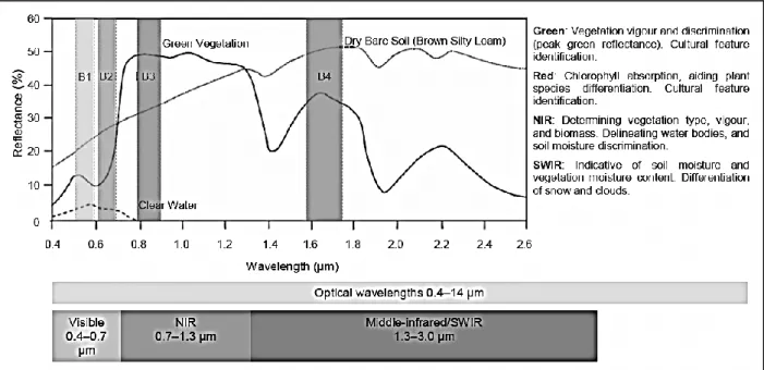
Figure 1: Spectral responses of common materials (Source: Clark, 2010)
Vegetation reflects at its minimum in the visible region, increasing sharply around 700nm (red edge) and highly in the near-infrared region. Soil and other bare surfaces comprise a steady increase across the visible and near-infrared spectrum (Clark, 2010). Clear water has a general spectral signature that peaks at around 400-500nm and exhibits total absorption in the near-infrared region. According to Jensen (2000) one of the distinct spectral responses of clear water is its absorption characteristic of almost all incident energy in the near-and middle-infrared (740-2500nm) portion of the spectrum. Most of the scattering occurs in the violet, dark blue and light blue categories (400-500nm) (Jensen, 2000). However, the
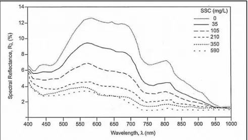
12 presence of organic and inorganic constituents complicates the normal spectral response of water. In-water constituents favor near-infrared surface reflection and sub-surface volumetric scattering thereby causing significant scattering and reflection (Jensen, 2000). They also shift the reflectance peaks towards longer wavelengths (Chen et al., 1992, Doxaran et al., 2002).
Such a characteristic is illustrated in Figure 2 below.
Figure 2: Change in reflectance against turbidity (After Chen et al., 1992)
The application of remote sensing in water resource management is not entirely new. In fact, aerial photographs, a form of remote sensing, have for decades been used to identify and examine water bodies (Krijgsman, 1994, Secor, 2006). Many studies have indicated that use of remote sensing techniques is more advantageous than traditional methods (He et al., 2008, Norsaliza and Hasmadi, 2010b). According to Zhengjun et al. (2008), remotely sensed datasets facilitate easier, rapid and seasonal water quality data collection at minimum costs.
Other studies note that remote sensing methods permit for more focused and efficient field sampling, potentially reducing the number of samples required for a particular water body (Adam et al., 2010, Hellweger et al., 2004, Secor, 2006).
The above mentioned advantages, together with the availability of established techniques and improved precision in atmospheric and geometric corrections, makes it possible to employ remote sensing to accurately assess and monitor water quality constituencies (Turdukulov, 2003). Many algorithms for data interpretations and modeling have been developed (Santini et al., 2010). Numerous studies have used remote sensing to estimate a range of parameters such as pH, salinity, chlorophyll-a, total phosphorus, temperature and total suspended
13 sediments (Chen, 2003, He et al., 2008, Norsaliza and Hasmadi, 2010a, Norsaliza and Hasmadi, 2010b, Pavelsky and Smith, 2009, Senay et al., 2001, Su et al., 2008b, Thiemann and Kaufmann, 2000, Volpe et al., 2011, Akbar et al., Undated, Wu et al., 2007). Whereas satisfactory relationships have been established for most marine water quality indicators, progress in inland freshwaters has been slow largely due to optical heterogeneity and turbid nature (Gons, 1999, Moore, 1980).
2.6.1 Estimating turbidity
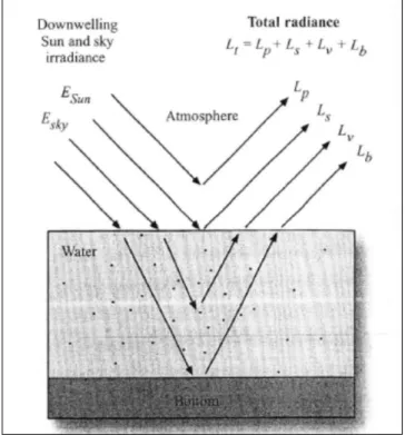
Moore (1980) notes the possibility of quantifying turbidity from remotely sensed measurements and highlights the importance of considering the principles of light and water interaction. Such an interaction is described by four sources of electromagnetic energy (Figure 3).
Figure 3: Sources of electromagnetic radiation (Source: Jensen, 2000)
As energy moves from the sun through the atmosphere, a portion of it is scattered and never reaches the water surface (Lp), while another portion manages to reach the air-water interface but barely penetrates the surface and is reflected away (Ls) (Jensen, 2000). This reflected energy may carry with it spurious surface reflectance due to wind-induced reflectivity and the presence of bubbles (Han and Rundquist, 1998). The portion that penetrates the water surface, reaches the bottom of the water body and then rises up to exit the water column, this
14 constitutes the bottom radiance (Lb) (Jensen, 2000). According to Jensen (2000) and Liu et al.
(2003) the later portion is useful for bathymetric or coral reef mapping. The portion that is crucial in water turbidity analyses is termed the subsurface volumetric radiance (Lv) (Koponen, 2006, Jensen, 2000). This portion manages to penetrate through the air-water interface, interacts with the water molecules and its constituents and then re-emerges from the water column without bouncing off from the bottom (Jensen, 2000). It is this portion that has valuable information about the characteristics of the water and its constituents and therefore useful in turbidity analysis (Jensen, 2000, Olet, 2010).
As aforementioned, water turbidity constituents include among others inorganic suspended minerals, organic chlorophyll-a and dissolved organic material (Jensen, 2000). Inorganic suspended minerals are a direct consequence of eroded material originating from among others upslope agricultural lands and weathered material (Jensen, 2000). These sediments commonly characterize inland waters and significantly influence spectral reflectance (Jensen, 2000, Miller and McKee, 2004). The presence of these materials affects the absorption and scattering coefficients differently at the various wavelengths. Re-radiated energy is propagated omni-directionally as a function of the size, refractive index and composition of the particles in the solution as well as the wavelength of the incident light (Omar and MatJafri, 2009, Sadar and Engelhardt, Undated). Smaller particles have a greater scattering effect on shorter wavelengths than on longer ones (Sadar, Undated). The reverse holds for larger particles.
2.6.2 Visible and Near-infrared regions
The visible region is reported as most useful in turbidity estimation (Lathrop and Lillesand, 1986, Norsaliza and Hasmadi, 2010b, Wang et al., 2006). Chen and Muller-Karger (2007) note a strong correlation at 645nm using MODIS Terra 250m data. Potes et al. (2012) found the best fit between water turbidity and the green/blue MERIS spectral band index.
Interesting features have also been noted in the near-infrared region. This region had previously received little attention due to pure water’s high absorption coefficient particularly in longer wavelengths (Doron et al., 2011). However, recent studies have noted that turbid waters, particularly those characterized by inorganic material, display a noticeable degree of reflectance following the presence of minerals (Doxaran et al., 2002, Ruddick et al., 2006, Shibayama et al., 2007). Good results have also been reported in turbidity estimation (Senay et al., 2001; Doxaran et al., 2002).
15 2.7 Methods of estimating water quality constituents
Existing literature distinguishes between analytical and empirical approaches for estimation of water quality constituents.
2.7.1 Analytical
The analytical approach makes use of bio-optical models, which basically capture the interactions between water and radiation (Koponen, 2006, Wong et al., 2008). This approach makes use of the inherent optical properties (absorption and backscattering) of water bodies to develop models. Once developed and verified, the models can be applied to any dataset regardless of its time of acquisition (Sugihara et al., 1985, Turdukulov, 2003). The main challenges with this approach are the assumption of an even distribution of water quality parameters within the water column, which may not hold in dynamic systems like rivers (Turdukulov, 2003). It also originates from a complicated computational procedure, which hampers its use and understanding.
2.7.2 Empirical
The empirical approach establishes a statistical relationship between the water constituent concentration and reflectance (Turdukulov, 2003). It forges a relationship between recorded spectral data and water quality parameter’s in situ data using a statistical method that seeks to minimize the error between the variables (Koponen, 2006). It can also be described as a method that utilizes experimental datasets and statistical regression techniques to develop algorithms that relate water-leaving reflectance to in situ measurements (Matthews et al., 2010). It is important to note that the development of algorithms requires concurrent acquisition of both in situ water quality samples and remote sensing data (Liu et al., 2003).
Such synchronization is important in capturing the temporal dynamics of water quality.
Resulting statistical relationships can take a simple linear, multiple linear or even non-linear character (Han and Rundquist, 1997, Koponen, 2006, Liu et al., 2003, Turdukulov, 2003).
The approach comes with its own pros and cons. The main drawbacks are that it is mostly limited to cases where in situ data is available and the resulting algorithms remain sufficient only for that particular dataset from which they were developed (Dekker et al., 1996, Koponen, 2006). This makes them not easily transferable to other areas or across seasons.
However, the method is accurate and easy to use (Koponen, 2006, Matthews et al., 2010).
16 2.8 Algorithm development
The development of algorithms essential for the prediction and estimation of water quality parameters requires statistical applications. There exist a variety of algorithms that are in use today. Some employ simple linear regressions between reflectance and water quality parameters (Koponen, 2006, Turdukulov, 2003, Liu et al., 2003). Others make use of multiple regressions (Ekercin, 2007).
The use of spectral indices in remote sensing studies has become popular since it was first initiated by Kauth and Thomas (1976) (Yamaguchi and Naito, 2003). Indices are very instrumental in converting spectral reflectance at specific wavelengths into biophysical information that can be easily interpreted (Shafique et al., 2003; Koponen, 2006). They essentially enhance the detectability of a particular parameter amongst others (Shafique et al., 2003). They are developed to improve parameter estimates. Several indices have been developed thus far, some for vegetation, soil and water detection. Generally bands, preferably adjacent, carrying the most information about the particular parameter of interest (usually the peaks and troughs of spectral reflectance graphs), are selected (Shafique et al., 2003). This involves analysis of the actual spectral plot for the peaks and troughs. Once the bands of interest have been identified, a series of indices can be derived using arithmetic computations such as band ratios, band differences, first derivatives of bands and/or a combination of ratios and band differences. Examples of these have been reported (Abd-Elrahman et al., 2011, Cairns et al., 1997, Duan et al., 2007, Koponen, 2006, Senay et al., 2001, Turdukulov, 2003, Turdukulov and Vekerdy, 2003, Arenz Jr et al., 1996, Han and Rundquist, 1997, Huang et al., 2010, Kutser et al., 2005, Östlund et al., 2001, Sudheer et al., 2006).
A common example to this is the normalized difference vegetation index (NDVI) first applied by Rouse et al. (1974). Since then many indices, new and modifications of existing ones, have been developed (Haboudane et al., 2004). Literature reports successful spectral indices in turbidity detection. Doxaran et al. (2002) obtained a convincing relationship with turbidity results when the ratio of near-infrared and visible bands was considered. This current investigation made use of these previous findings to guide the current exploration (Chen et al., 2009, Senay et al., 2001, Turdukulov, 2003). A recent addition is the use of derivatives of measured spectra in developing algorithms, which together with band ratios have been considered key in separating spectral effects of different water constituents (Giardino et al., 2007, Han and Rundquist, 1997, Turdukulov, 2003).
17 Most of these applications have been applied mostly over ocean water where the major optically active constituent is chlorophyll. However, radiation in inland freshwater bodies comprises of complex energy interactions due to the presence of other constituents. This results in considerable scattering and can complicate the relationship between measured spectra and measured constituent’s concentrations (Sudheer et al., 2006).
2.9 Summary
Deteriorating water quality is a global problem. Generally, turbidity limits water’s utilization value, adds on water treatment costs and induces disease outbreaks. Consequently, turbidity measurement helps monitor water quality which play an important role in detecting the impacts of agricultural and urban sediment loads on water resources. With notable advancements in remote sensing such as spectral improvements, it is now possible to use remote sensing to detect turbidity. Empirical methods that establish a relationship between recorded radiation energy and measured turbidity play an important role in water turbidity detection. However, most of the work done is over ocean waters. Little has been reported on inland freshwater bodies largely due to the complex energy interactions caused by suspended materials. It is therefore important to explore and select optimal spectral bands suitable for turbidity detection.
18 CHAPTER 3: RESEARCH METHODOLOGY
3.1 Introduction
This chapter details the methods employed in this study to realize the objectives outlined in Chapter 1. It summarizes how spectral reflectance and corresponding turbidity readings were measured at different levels of soil in an amount of water. It also explains the methods of analysis adopted to ascertain answers to the question of optimal spectral bands for turbidity determination.
3.2 Data acquisition and methods
To achieve the set objectives as outlined in Section 1.3, the study selected a suitable area from which soil samples were collected. These were used to create different levels of turbidity through mixing a known amount of soil material in a known volume of water. It was from these mixtures that the respective spectral reflectance together with the corresponding laboratory based turbidity data, were collected. The data collected was analyzed to explore the connection between turbidity and spectral reflectance and also identify optimal spectral bands in turbidity estimation. The methods adopted in data collection and analyses are elaborated upon.
3.2.1 Study area
The soil samples used in this study were localized along the bank of the Msunduzi River in the Pelham area, Pietermaritzburg. The site is gently sloped with minimal topographic variations that are attributed to the river’s history of dredging and associated silt deposition (Singh, 2010). The site falls within an area that is currently being used as a recreational park area. There’s moderate vegetation cover with a distinct avenue of trees along the river. The river has a turbid character following upstream and surrounding erosion of soil and other contaminants. It flows in a west east direction. To mimic the turbidity characteristics of the river, it was deemed necessary to collect soil sample material close to the river. A locality map, showing the sample points with the latest aerial photograph underlay, was prepared and is presented in Figure 4.
19 Figure 4: The distribution of sample sites in the study area
3.2.2 Soil samples
Samples were sited using a systematic random sampling approach separated by an approximate distance interval of 40 meters (Figure 4). Since the focus of the study was not on the impact of different soil types in turbidity but rather on the amount, the siting of the sample sites at specified distances was meant for data separability not soil type differences.
An approximate mass of 3 kilograms of soil was collected at each of the 15 sampling sites and then oven dried over night at 105oC. This temperature is recommended as it does not alter the chemical and physical attributes of the soil (Carter and Gregorich, 2008). After drying, the collected samples were gently crushed and passed through a 2mm diameter mesh sieve. The sieved soil samples served as input for the turbid solutions from which both the laboratory and spectral reflectance measurements were performed. Using an electronic scale, 15 different mass levels incremented by 10 grams (g) (i.e 10g, 20g, 30g…150g) were weighed out from each sieved soil sample. Weighing these samples was important in creating solutions of different turbidity levels. The resulting masses were secured in sealable plastic bags. This exercise generated a total of 225 soil replicates, 15 for each mass level. An
20 approximate mass of 460g from each sample was taken to the Department of Agriculture and Environmental Affairs in Cedara, KwaZulu-Natal for determination of chemical and physical characteristics (Table 2).
3.2.3 Spectral measurements of turbid solutions
The 255 weighed sieved soil masses were used to prepare turbid solutions upon which the spectral measurements were to be conducted. Spectral reflectance data was collected using a 350 to 2500nm Analytical Spectral Device (ASD) field spectroradiometer (FieldSpec®, Analytical Spectral Devices, Inc., US) in the field. The ASD device records radiation at 1.4- nm intervals and 2-nm intervals for the spectral regions 350 to 1000 nm and 1000 to 2500 nm, respectively. Data were interpolated to 1-nm spectral resolution across the spectrum. To minimize bi-directional influence as per changing sun angle, measurements were taken under clear sunlight between 10 am and 14 pm. Prior to data collection, the spectrometer was calibrated to respective spectral measurement lighting conditions using a Spectralon white reference panel. The validity of the calibration was tested using the panel’s reflectance.
During spectral measurement, calibration was repeated after an average of 30 spectral scans were collected or when the instrument reached saturation. Care was taken not to handle or expose the panel to dirt, water or any other damaging substance during and after calibration.
Two 1000 milliliters glass beakers of 10.5 cm diameter and 14.5 cm depth were used to hold samples for spectral measurements. The first beaker was wrapped with a black plastic liner so as to limit light interference from the surroundings (Lodhi et al., 1997, Karabulut and Ceylan, 2005). The second beaker was unlined and used to mix the different turbid concentrations.
Each sieved soil mass increments (i.e 10 to 150g) was transferred into the unlined 1000ml glass beaker, one at a time, together with a litre of deionized water and stirred to make a turbid solution. Deionized water was preferred so as to minimize the possible influence of any dissolved salts in water on the reflectance. The solution was then transferred into the lined beaker, filling it up to the 1000ml mark with the solution, for spectral measurements.
The sediment was kept in suspension by manually stirring so as to ensure the homogeneous distribution in the water. The solution was given a brief delay prior to scanning to avoid wave effects. Once ready the 1 degree field of view (FOV) head attached to a fibre optic pistol was positioned at about 10cm directly above the water surface and the spectral reflectance measurement taken. To avoid spectral contamination, care was taken to ensure that only the
21 spectral reflectance of the water solution covered by the FOV was recorded. An average of 15 scans ranging from 350-2500nm wavelength range within the electromagnetic spectrum was taken. The spectral reflectance of deionized water (0 g/l) was also collected so as to quantify the signature of pure water. The same procedure was followed to record the spectral reflectance of the rest of the prepared turbid solutions at the different concentration levels (10g/l, 20g/l, 30g/l, 40g/l, 50g/l, 60g/l, 70g/l, 80g/l, 90g/l, 100g/l, 110g/l, 120g/l, 130g/l, 140g/l and 150g/l).
3.2.4 Laboratory turbidity measurements
The laboratory based turbidity measurements were carried out using a 2100Q portable turbidimeter (Hach Company. Loveland, Colorado). This instrument makes use of a tungsten filament lamp source and a silicon photodiode detector to determine the amount of particles in the solution. After an initial calibration, the turbidity measurement is achieved by turbidimetric ratio determination using a primary nephelometric light scatter signal positioned at 90o to the transmitted light scatter signal. Typically, the device is battery powered with a measurement range of 0 to 1000 Nephelometric Turbidity Units (NTU). It has a resolution of 0.01 NTU and an accuracy of ±2% of reading plus stray light (≤ 0.02). Due to instrument unavailability, the turbidity measurements were sourced out to a nearby water testing agency, Talbot & Talbot (Pty) Ltd. As part of the agency’s regulation, a volume of 500ml of the turbid solution is required for turbidity measurements. This ensures that analyses can be repeated if and when errors are encountered.
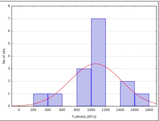
Laboratory based turbidity measurements were carried out from the same type of turbid solutions created from mixing each of the weighed sieved masses with deionized water, thus creating turbid solutions of different concentrations as in Section 3.2.3. These were thoroughly mixed and then half the solution (500ml), as required by the water testing agency, transferred into 500ml sealable plastic bottles to be sent for laboratory analysis. It is noted though that due to the project’s limited funds only 149 out of the 255 prepared turbid solutions was analyzed for laboratory turbidity (see Table 2). This number covers approximately 11 of the primarily 15 initially collected soil samples.
Prior to analyses, the agency subjected each of the 500ml solutions to gentle shaking to facilitate homogeneity. From these solutions, 15ml aliquots were extracted using a sample
22 cell from which the turbidity values were to be measured. A thin film of silicon oil was applied over the entire surface of the sample cell to mask the sample cell’s minor imperfections and scratches that may contribute to light scattering. Thereafter the turbidity values were measured from the extracted 15ml aliquots within 24 hours of mixing to minimize the influence of any possible organic or chemical reactions, and then measured data transferred into an MS excel spreadsheet and basic statistics computed. In cases where the turbidity value exceeded the instrument’s high limit (i.e 1000 NTU), the extracted aliquots would be diluted with Type 1 Milli-Q water (ultrapure grade water) to acceptable ratios, then the turbidity would be measured from the resulting solution and the resulting value multiplied by the factor of dilution to get the turbidity value of the original solution.
3.3 Processing
3.3.1 Initial spectra processing
Using the ViewSpec ProTM spectra viewing software, the collected spectra were explored and mean spectra at each wavelength computed. The computed files were converted into ASCII text files readable in MS Excel. The spectral range was limited between 400 to 1000 nm firstly because noise became a problem at wavelengths beyond this spectral range. Secondly, literature reports this range as the most appropriate for turbidity detection (Norsaliza and Hasmadi, 2010a, Senay et al., 2001, Wang et al., 2006). It was also noted that water displays interesting spectral responses in the said range, particularly the near-infrared region and therefore the study sought to investigate its relevance to turbidity detection. Reflectance was computed as the ratio between reflected energy from the water surface and the Spectralon white reference panel.
3.3.2 Estimating turbidity
The relationships between the raw spectral reflectance in the 400 to 1000nm range and laboratory based turbidity measurements were tested using the Pearson’s coefficient of correlation (r) with a significance of p<0.05. The test yielded poor results with its highest coefficient being 0.4. The study therefore opted to compute the mean spectral reflectance (denoted by X10 to X150) at each of the turbid solution’ concentration level (i.e. 10g/l up to 150g/l). This helped compensate against noise and also enhanced variability between the different turbidity levels.
23 The resulting spectra were explored for the strongest and most appropriate band/s per spectral portion (i.e. blue, green, red and near-infrared) in turbidity detection using Pearson’s coefficient and simple regressions. It was important to partition the bands according to their
“natural” regions because of their unique characteristics and behavior in water. Jensen (2000) explains the roles of the different regions, pointing out the usefulness of the visible and near- infrared regions in providing information about the type of soil and amount in suspension, respectively. This partitioning helped reduce the probability of selecting bands containing the same information (i.e. data redundancy) as a result of inter-band correlation. The study also explored for optimal spectral indices using the same criteria as single bands above. As mentioned in Section 2.8, spectral indices enhance the detectability of a particular parameter and also improve parameter estimates (Shafique et al., 2003). The exploration involved first derivatives of reflectance, band differences, band ratios and combination indices. Their associated formulae are presented in Table 1. Most of the indices explored were traced from previous turbidity studies.
Table 1: Formulae for spectral indices
Index type Computation References
Simple ratio Ri / Rj Koponen (2006), Shafique et al.
(2003), Potes et al. (2012) First derivative (Ri - Rj) / (λi - λj) Senay et al. (2001)
Band differences Ri - Rj Shafique et al. (2003)
Normalized indices (Ri - Rj) / ( Ri + Rj) Shafique et al. (2003)
where Rj and Ri represent the spectral reflectance at band i and j, and λi and λi are the band wavelengths at band i and j.
Using regression analysis, the best bands, per spectral portion (blue, green, red and near- infrared), were selected noting their respective Pearson’s coefficient of correlation and the resulting coefficient of determination (R2) with measured water turbidity. Bands that yielded the highest R2 values against turbidity constituted the best bands. The study selected the best 3 bands, as informed by Mutanga and Rugege’s (2006) method, from each spectral category (i.e. blue, green, red and near-infrared), and using the highest R2 criteria after cross validation as explained below, the best band, in each spectral category, was noted. These are also treated as representative bands for each of the spectral categories. There was a slight variation in the near-infrared region. An additional band was included in this category, thereby making a total
24 of 4 bands. The reason behind the additional band is informed by the wideness of the near- infrared region. It was observed that one end of the region is dominated by high reflectance while the other by low reflectance (see Figure 7). It was therefore interesting to see how these differences would impact the strength of the relationship with turbidity. Furthermore, 2 spectral indices, one from each region (i.e. visible and near-infrared), were selected. In the end a total of 13 best single bands plus 2 spectral indices were extracted, thereby making a total of 15 variables.
3.3.3 Model validation
The usefulness of values estimated with remote sensing is very limited without proper indications of their accuracy. The study computed regression models between the observed and predicted values of turbidity and then subjected resulting models to a validation process using the leave-one-out cross-validation (LOOCV) procedure. The LOOCV technique isolates a single observation for validation purposes and then uses the rest of the observations as training data. This was done for all of the observations. The resulting model was then used to predict the previously isolated observation. In each iteration, adjusted R2 and root mean square error (RMSE) values were recorded and later the mean values of each computed. The RMSE value and the adjusted R2 were calculated by relating the predicted value generated during the LOOCV procedure to the observed value so that the accuracy of turbidity estimation can be ascertained. The technique is widely used in remote sensing and well suited for small sample sizes (Wang et al., 2013, Sterckx et al., 2007). Models with the highest R2 and the lowest RMSE were considered as optimal.
3.4 Summary
A total of 15 soil samples were collected in the study site, oven dried, sieved and replicates extracted. The replicates, with masses ranging from 10 to 150g, were each mixed with deionized water to create turbid solutions over which spectral reflectance together with laboratory based turbidity values were measured. The basic soil chemical and physical characteristics were also determined. Thereafter, the spectral data was explored for the strongest relationships with measured turbidity and then R2 value reported. Models were cross validated using the LOOCV procedure, reporting both the RMSE and adjusted R2.Such exploration was limited to the visible-near infrared region of the spectrum. A few spectral bands displayed strong relationships with turbidity.
25 CHAPTER 4: RESULTS
4.1 Introduction
As set out in Chapter 1, this study sought to investigate the relationship between turbidity levels and spectral reflectance and then move on to identify the optimal bands that can be used to estimate turbidity. Consequently, this chapter presents results from the soil analysis, laboratory based turbidity measurements, spectral reflectance measurements and the investigation to identify optimal bands that correlated best with turbidity measurement.
4.2 Soil properties and reflectance
Soil attributes play a significant role in the amount of electromagnetic energy reflected or absorbed (Rossel et al., 2006). Demattê et al. (2010) note a close relationship of soil attributes such as organic matter with reflected energy. Other studies have explored this connection by using visible near-infrared spectroscopy to predict organic carbon, nitrogen, clay content, exchangeable calcium, micronutrients and others (Bilgili et al., 2010). Jensen (2000) notes a distinction in reflectance between silty and clayey soil, reporting higher reflectance values in the visible region for silty soils in comparison to all other wavelength regions.
The soils used in this study were predominantly clay loam, darker in colour with a significant amount of organic matter and clay (Table 2). There was little variation in soil attributes as sampling was localized around the same area.