Clamping force It is the force applied to the mold by the clamping unit of the injection molding machine during the filling, packaging and cooling phases of the molding cycle, measured in tons. Polymers have high coefficients of thermal expansion and significant shrinkage occurs as the plastic cools in the mold.
Objectives of this Investigation
In Chapter 5, an alternative model for the build-up of cooling stress in an injection-molded part is proposed. The role of both pressure history in the molten polymer during cooling, and the interaction between the sample and the mold is identified and numerical calculations of the final cooling stress distribution are performed.
Literature survey
Darlington et al [13] investigated the pressure loss in the mold during the packaging stage of the injection molding process. A computer software package (COOL3D) was developed for the simulation of heat transfer during the cooling stage of the injection molding process.
Available Commercial Systems
They performed a coupled analysis of the fluid flow and heat transfer in the molten polymer during the filling and post-filling stages of the injection molding process, and of the mold cooling that occurs throughout the process. One of the performance simulations that CAD can provide includes the Injection Molding Simulation software program C-MOLD, a widely used polymer processing operation.
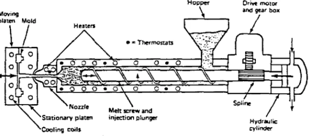
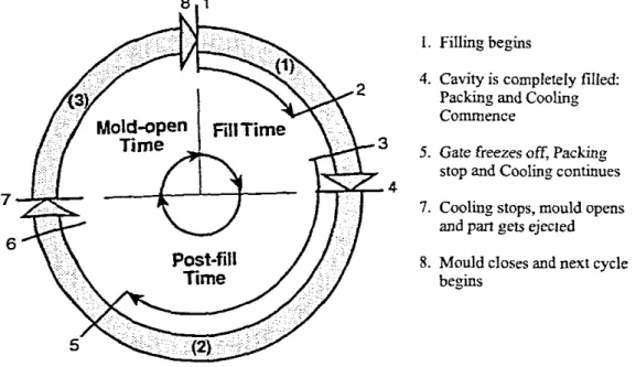
Introduction to the Injection Moulding Process
The residual stress resulting from the change in thickness of the part is then the induced stress. The melt temperature refers to the temperature of the polymer in the barrel just before injection.
Overview of thennal transfer
Modelling of the Time-varying Component (T m,J
The time-varying components at this interface cannot be considered zero due to the thermal impulse due to the hot polymer.
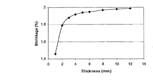
Sensitivity Analysis of Shrinkage
- The Process Estimator
- Varying Thickness
- Varying Fill Time
- 1 rrm Thickness I _'551
- Varying Melt Temperature
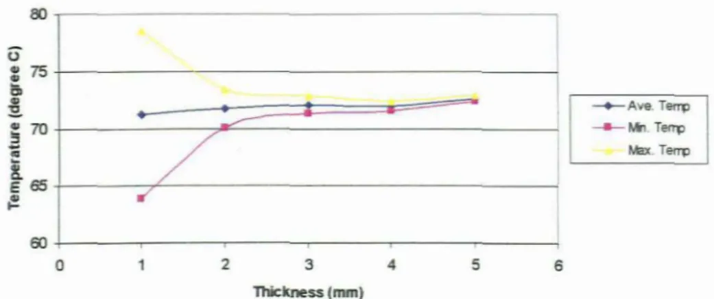
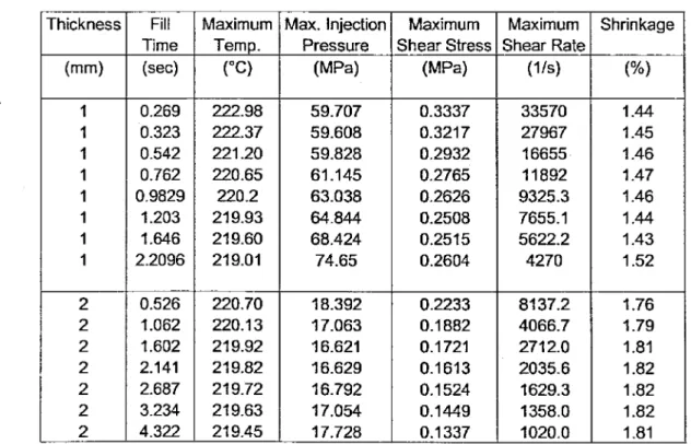
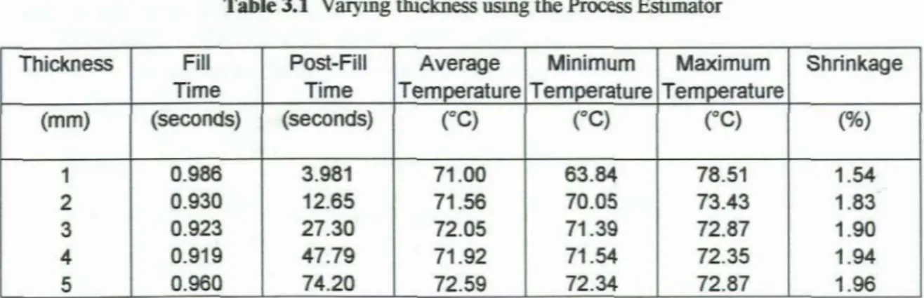
Note that the refill time refers to the duration of the refill time and not the time at the end of the refill phase. The average, minimum and maximum temperature columns in Table 3.1 refer to the component temperature at the end of backfill and are across the width-length of the cavity and not across the thickness direction. The thickness of the sample was constant at 3 mm, with the injection temperature constant at 220oe.
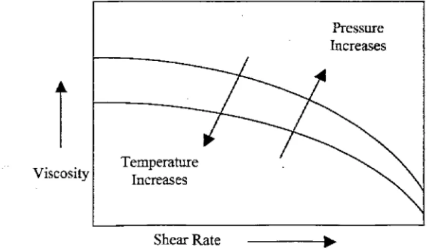
The shrinkage percentage value obtained from C-MOLD for polystyrene (Table 3.4) is relatively low compared to the values for polypropylene and polyethylene. Very slow filling times lead to excessive cooling of the melt front resulting in an increase in shear stress. This deviation from the norm can be attributed to the fact that there is an improved packing caused by the ram effect of the fast-moving molecules [25].
An increase in the melting temperature means an increase in the mobility of the molecular chains of the polymer, leading to a decrease in shear stress.
Injection Moulding Analysis Case Study
- Background
- Filling Process
- Process Parameters and Packing
- Cooling System
- Shrinkage and Warpage
- Analysis and Discussion of Results
- Conclusions
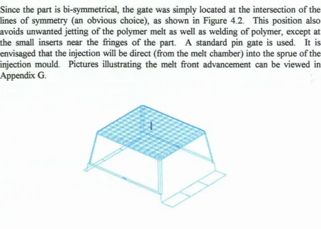
It is envisaged that the injection will be directly (from the melting chamber) into the injection molding of the injection mold. Weld lines can be observed in the part due to the inserts in the flow region. At the end of the filling stage, the inlet pressure is kept constant (during the refilling or packing stage), so that the cavity can be compacted.
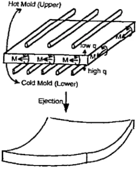
The temperature distribution along the part (mass average) at the end of the cycle time or at the ejection point is given in Figure 4.5. Shrinking and twisting of the part (that is, the total deviation of the part from the original) is shown in two views in Figure 4.7. Visual inspection shows the degree of shrinkage (which is normal) and the associated deformation of the part.
At this stage, the bias in the center of the lot is the downward y-direction of concern.
ChapterS
An Alternative Model for the Stress Build-Up during Cooling of Injection Moulded Thermoplastics
Introduction
These suggest that features such as interaction of the polymer with the mold and pressure history in the melt play a very important role. According to the choice of reference, x is related to the Euclidean space of physical perception and indicates the current position of the material element in question. This similarity is due to the choice of the spatial (Eulerian) or material (Lagrangian) representation, respectively.
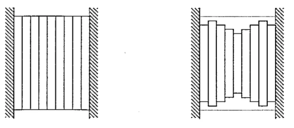
The fourth faces of the polymer and mold will be referred to as edges and the remaining two larger faces as walls. The temperature distribution of the molten polymer at the end of filling, when packaging begins, is assumed to be uniform. If the pressure in the molten polymer and the adhesion of the part to the mold walls are negligible, the part undergoes free quenching.
Under such conditions, the part will undergo continuous longitudinal shrinkage due to the effect of thermal contraction of the layers, from the solidification temperature to the wall temperature.
Governing Equations
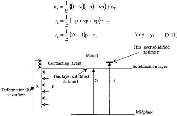
At any time, the stress. distribution in the solid shell lying on the mold walls must be in balance with the external forces acting on it. These forces are related to the melt pressure that pushes the solid polymer against the mold, and the interaction between the solid polymer and the mold. Referring to the solid layer at the solidification temperature Ts, the stress along a direction x perpendicular to y can be written as.
As long as the pressure in the melt remains positive, the solid layer is held against the mold walls. At the solid-melt interface, solidification occurs under hydrostatic pressure, so that all three stress components are equal to the hydrostatic pressure (-p) at this time. Only the interaction between the solid polymer and the mold edges is considered, as it prevents the sample from exceeding its original dimensions.
The melt pressure stretches the solid shell through the force acting on the edges of the sample.
Discussion of Results
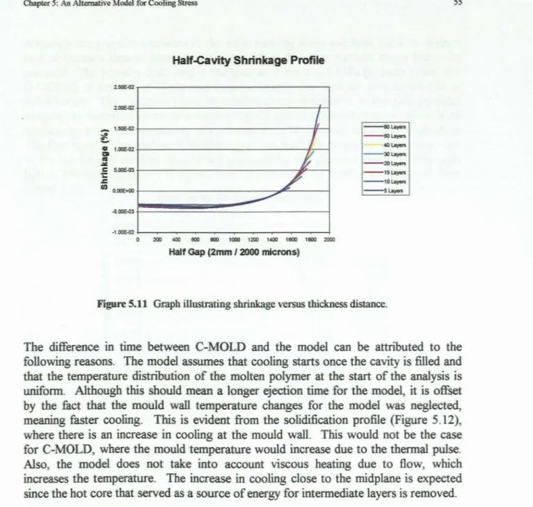
The model assumes that cooling starts when the cavity is filled and that the temperature distribution of the molten polymer at the start of the analysis is uniform. The signature curve of cooling stress distribution in injection molded specimens, as described in the introduction, would not be obtained because there is no pressure rise immediately after filling, as in injection molding in practice. The first layer of the analysis is positive as the model is proposed in such a way that the behavior of the first layer is not controlled by any previous layer.
From figure 5.15 we notice that the curve for the final cooling stress for the number of layers has converged. Including the effect of a thermal pulse in the ABAQUS analysis to account for the mold wall temperature rise would be required for more accurate calculation results. Practical experiments regarding material and process parameters would however allow better testing of the model, especially the determination of the pressure field.
An agreement between the numerical model and the commercial software could not be found due to the lack of information about the model parameters and approximations.
Conclusions
- Concluding this work
- Future Work
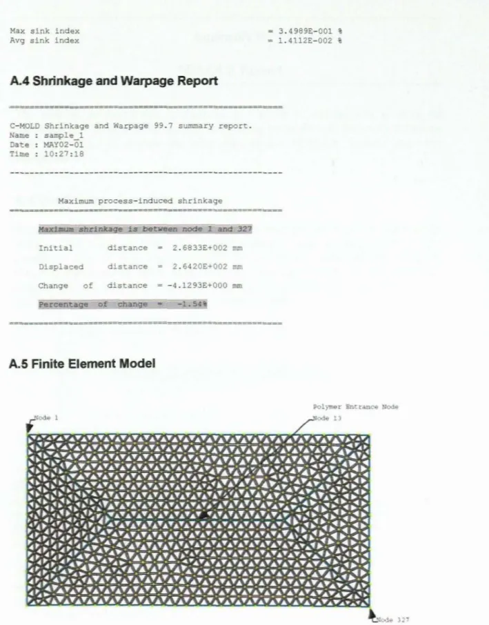
- Shrinkage and Warpage Report
- Finite Element odel
H., (1989), Numerical simulation and experimental investigation of melt solidification injection mold filling, Polymer Engineering and Science, (V. 29), p. K., (1993), Integrated Simulation of Fluid Flow and Heat Transfer in Injection Molding to Predict Shrinkage and Curl, Joumal of Engineering Materials and Technology, (V. 115), p. F Finite element/finite difference simulation of the injection filling process, Journal of Non-Newtonian Fluid Mechanics, (V. 7), p.
28] Jacques, M., (1982), An analysis of thermal distortion in injection molded flat parts due to unbalanced cooling, Polymer Engineering and Science, (V. 22). G., (1986), A Structure-Oriented Computer Simulation of Injection Molding of Viscoelastic Crystalline Polymers Part I: Model with Fountain Flow, Packing, Solidification, Polymer Engineering and Science, (V. 26), pp. G., (1986), A Structure-Oriented Computer Simulation of Injection Molding of Viscoelastic Crystalline Polymers Part 11: Model Predictions and Experimental Results, Polymer Engineering and Science, (V. 26), p.
C., (1990), An Improved Flow Analysis Network(FAN) Method for Irregular Geometries, Polymer Engineering and Science, (V. 30), bl.
AppendixB ABAQUS Report
The Problem Description
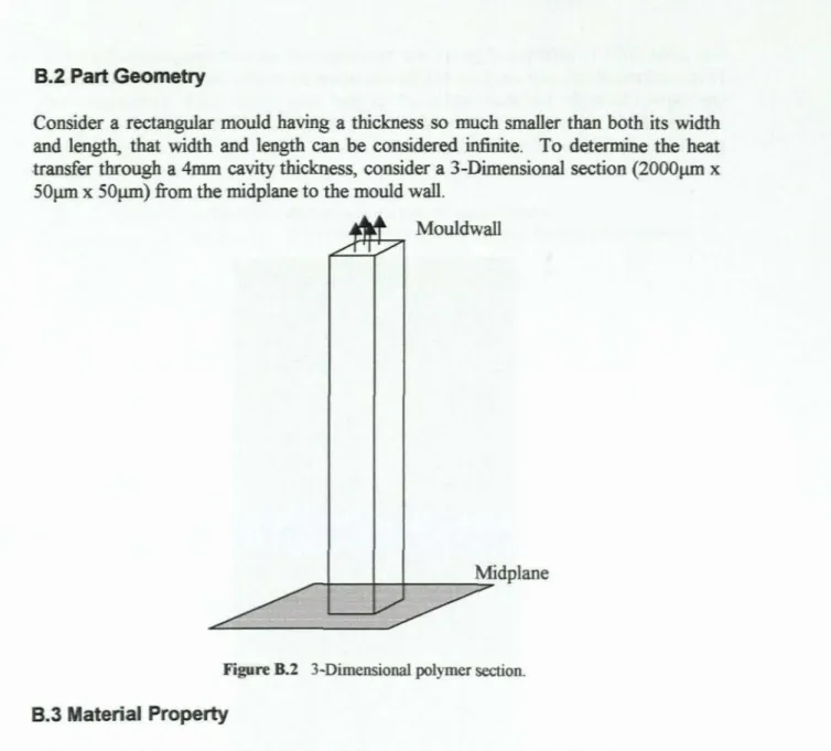
- Part Geometry
- Material Property
- Analysis Step
- Interaction
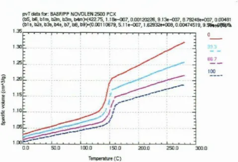
All material properties come from the database of the injection molding simulation software C-MOLD. Since the main purpose of this analysis was to determine the temperature field, extra attention had to be paid to the thermal properties. Latent heat is the heat absorbed when a substance changes phase from liquid to solid [18,23], and in the case of the injection molding process it is called solidification.
When we see the specific heat versus temperature graph (Figure BA) of Borealis, a definite increase in the .. specific heat can be seen at the transition temperature. A boundary condition is set for the surface at the midplane and along the four surfaces for the length of the section. However, the polymer's loose heat at the mold wall surface to the surrounding tool steel and the thermal conductivity of the tool steel and the heat transfer across the joint must be taken into account.
Since it is assumed that the air that originally filled the cavity is vented and the entire cavity is filled with polymer, the cavity area and thermal conductivity of the cavity fluid drop out. This results in an equal contact area and a total surface area.
Load
It is assumed that the polymer loses heat through contact conduction with the mold wall surface. The physical mechanism of contact conduction can be better understood by examining a joint in more detail. No surface is perfectly smooth, and the surface roughness plays a central role in the transfer of heat.
The surface of an injection molding cavity is polished to a very high degree; from 10 ftIIl to as low as 1 J.l1ll [26]. The results obtained for the contact coefficient are entered as the film coefficient in ABAQUS. Since mold wall temperature changes were assumed to be negligible, the mold wall for the tool steel is set at a constant temperature of 40QC.
Meshing
Appendix C ABAQUS Output Data
AppendixD FORTRAN Program
AppendixE FORTRAN Results
MOLD Output Data
- Log File
Comparisons are made between the cooling and shrinkage times for C-MOLD and the cooling and shrinkage times for the numerical model proposed in Chapter 5. The input and output data for the C-MOLD analysis can be found in this Appendix. The separation plane is not specified; the default parting plane .. normal along the Z axis of the global coordinates will be. The analysis will be based on {I) Parameters : .. of layers along the full void .. design results in post-fill .. results detailed in convergence criterion of melting temperature after filling Kid).
Average aspect ratio of 20 elements Maximum aspect ratio of 2D elements 2D element number wl maks~ aspect ratio Minimum aspect ratio of 2D element 20 element number w/min.
AppendixG
Melt Front Advancement
AppendixH Part Performance