i
Selective production of difluorodimethyl ether from chlorodifluoromethane – A kinetic study using a well-mixed batch absorber
Rasmika Prithipal [BSc. Eng]
In fulfillment of the requirements for the degree Master of Science in Engineering, Chemical Engineering,
University of KwaZulu-Natal
March 2013
Name of supervisor: Prof. D. Ramjugernath Name of co-supervisor: Prof. M. Starzak
ii
As the candidate’s Supervisor I agree/do not agree to the submission of this thesis.
_________________________________ _________________________________
Prof. D. Ramjugernath Prof. M. Starzak
DECLARATION
I ………. declare that
(i) The research reported in this dissertation, except where otherwise indicated, is my original work.
(ii) This dissertation has not been submitted for any degree or examination at any other university.
(iii) This dissertation does not contain other persons’ data, pictures, graphs or other information, unless specifically acknowledged as being sourced from other persons.
(iv) This dissertation does not contain other persons’ writing, unless specifically acknowledged as being sourced from other researchers. Where other written sources have been quoted, then:
a) their words have been re-written but the general information attributed to them has been referenced;
b) where their exact words have been used, their writing has been placed inside quotation marks, and referenced.
(v) Where I have reproduced a publication of which I am an author, co-author or editor, I have indicated in detail which part of the publication was actually written by myself alone and have
fully referenced such publications.
(vi) This dissertation/thesis does not contain text, graphics or tables copied and pasted from the Internet, unless specifically acknowledged, and the source being detailed in the
dissertation/thesis and in the References sections.
Signed:_______________________________
iii
Acknowledgements
To my parents, Anil and Lalitha Prithipal, and my sister, Arisha Prithipal, thank you for your love, support, and words of encouragement.
I would like to thank Prof D. Ramjugernath for affording me the opportunity to work on this project. Sincere thanks to Prof M. Starzak for his time, constant guidance and knowledge throughout the project. I would also like to thank Dr. David Lokhat for his assistance and guidance.
It is greatly appreciated. Many thanks extend to Prof. J.D. Raal for his assistance with the thermodynamic derivation and to Dr. Daniel Teclu for kindly imparting his knowledge of solution chemistry. I would like to also thank the technical staff at the School of Chemical Engineering:
Rekha Maharaj, Sadha Naidoo, Dudley Naidoo, Merlien Reddy, Danny Singh, Thobekile Mofokeng, Preyothen Nayager and as well the workshop staff, for their much needed assistance, experience and willingness to help. Sincere gratitude is expressed towards the Pollution Research Group: Dr. K.M. Foxon, Mr. C.J. Brouckaert and Kavisha Nandhlal for the dissolved oxygen probe used in this project. I am also thankful to Bilal Kazi for kindly assisting me in the laboratory. To all my friends, thank you for your great company and the good laughs we shared through trying days.
Lastly I would like to thank the National Research Foundation (NRF) for their financial support.
iv
ABSTRACT
The gas-liquid reaction between chlorodifluoromethane (R-22) and methanol, in the presence of sodium hydroxide, was investigated in an isothermal, stirred, semi-batch reactor. The objective of the study was to develop a model for the reaction and to identify the kinetic parameters. Reactor temperature was varied from 283 to 303 K, with inlet R-22 partial pressures between 40.5 and 60.8 kPa (absolute). Solutions containing sodium hydroxide concentrations of between 1.5 and 2.5 mol·dm-3 were charged into the reactor prior to each experiment. Preliminary investigations using the R-22-methanol system revealed that stainless steel was an inappropriate choice of material for the reactor as it displayed catalytic tendencies toward trimethyl orthoformate formation.
Consequently, the reactor was constructed from glass and was equipped with an internal cooling coil, a single heating jacket and a temperature control unit. Liquid samples that were withdrawn from the reactor were degassed under vacuum to remove residual chlorodifluoromethane, and thereby inhibit further reaction. Spectrophotometry was used to analyze the liquid samples to determine the concentration of chloride ions in solution. The products obtained were difluorodimethyl ether (major product) and trimethyl orthoformate (by-product) as well as sodium chloride and sodium fluoride salts. Difluorodimethyl ether is a potential replacement for ozone depleting CFC refrigerants. A Box-Behnken experimental design was used to investigate the effect of reaction conditions on the product distribution. Variations in the reaction temperature, initial concentration of sodium hydroxide and inlet partial pressure of R-22 were considered.
The modeling of the gas-liquid reactions was based on the -dehydrohalogenation mechanism.
Since gas solubility in a liquid decreases in the presence of dissolved salts, the "salting-out" effect on mass transfer was included in the reactor model. Sechenov coefficients for sodium chloride and sodium fluoride were combined to give a salt Sechenov coefficientKsalt. It was known from the literature that the presence of precipitated salts causes inefficient mixing and inhibits mass transfer, particularly in this system due to the relatively low salt solubilities in methanol. This mixing effect was also included in the appropriate mass transfer terms of the reactor model. The experimental data was fitted to a proposed kinetic scheme. Kinetic parameters for each of the proposed reactions, the Sechenov ‘salting out’ coefficients and the mixing parameter were obtained through the use of a non-linear, least-squares optimization algorithm. For the kinetic study, activation energies of 89.12 and 45.83 kJ·mol-1 were obtained for the difluorodimethyl ether and trimethyl orthoformate formation reactions, respectively, with a Sechenov salt coefficient of 0.712 and a mixing parameter of 22.43.
v TABLE OF CONTENTS
List of Figures………..ix
List of Tables………...xviii
Nomenclature………xxi
CHAPTER 1: INTRODUCTION 1.1. Background and motivation……….1
1.2. Objectives……….2
1.3. Thesis outline………2
CHAPTER 2: LITERATURE REVIEW 2.1. Fluoroorganic compounds: characteristics………...4
2.2. Chemistry of ozone destruction………6
2.2.1. Ozone depleting potential……….7
2.2.2. Global warming potential……….8
2.3. Properties and characteristics of refrigerants………...11
2.3.1. Physical properties……….11
2.3.2. Chemical properties..……….11
2.3.3. Thermodynamic properties...12
2.3.4. An ideal refrigerant………12
2.4. Substitution of chlorine containing fluoroorganic compounds with HFEs...13
2.5. Dechlorination of R-22 with methanol………...14
vi
2.5.1. Reaction schemes………...14
2.5.2. Experimental studies of difluorodimethyl ether production from R-22…….17
2.6. Analytical methods……….20
2.6.1. Determination of chloride ion concentration………..20
2.6.2. Determination of fluoride ion concentration………..23
CHAPTER 3: THEORY 3.1. Model of reaction chemistry………...28
3.2. Kinetic modeling……….………...29
3.3. Reactor model……….30
3.3.1. Material balances………30
3.3.2. Gas solubility……..………36
3.3.3. Mass transfer coefficient.….………..37
3.3.4. Enhancement factor………41
CHAPTER 4: EXPERIMENTAL 4.1. Equipment………...46
4.1.1. Preliminary testing on semi-batch reactor systems………47
4.1.2. Batch absorber for the R-22-methanol kinetic study………..58
4.1.2.1. Setting the feed gas composition………...58
4.1.2.2. Reactor vessel……….……59
4.1.2.3. Reactor temperature control system………...61
4.1.2.4. Vacuum degassing rig………63
vii
4.1.3. Apparatus for the measurement of (kLa)oxygen...65
4.1.3.1. Setup for (kLa)oxygen tests………65
4.1.3.2. Rig for the determination of the sensor lag………66
4.2. Materials and Procedures………67
4.2.1. Feed preparation……….67
4.2.2. Calibration………..68
4.2.2.1. Rotameter calibrations………68
4.2.2.2. Temperature sensor calibration………..69
4.2.2.3. GC Calibration….……….72
4.2.3. Experimental Procedure……….73
4.2.3.1. Procedure for preliminary experiments………..73
4.2.3.2. Procedure for the R-22-methanol kinetic study……….75
4.2.3.3. Procedure for the dissolved oxygen sensor lag measurements…..76
4.2.3.4. Procedure for (kLa)oxygen measurements...…..76
4.3. Analytical………77
4.3.1. Preparation of reagents………...79
4.3.2. Preparation of standard solutions for the calibration of the spectrophotometer………....79
4.3.3. Calibration of spectrophotometer………...80
4.3.4. Pre-preparation of samples for spectrophotometric analysis……….80
4.3.5. Preparation of samples for spectrophotometric analysis………81
4.3.6. Procedure for analysis………81
4.4. Experimental Design………..82
viii
4.4.1. Preliminary tests using the OVAT approach………82
4.4.2. Experimental design for the kinetic study..………..83
CHAPTER 5: RESULTS AND DISCUSSION 5.1. Preliminary experiments……….86
5.2. Raw experimental data...……….93
5.3. Nonlinear data regression………...96
5.4. Total salt concentration controversy………...97
5.5. Parameters of the Arrhenius equation………....98
5.6. Salting-out coefficients of the Sechenov equation……….99
5.7. Results of isothermal data fitting………..101
CHAPTER 6: CONCLUSIONS AND RECOMMENDATIONS 6.1. Conclusions………..122
6.2. Recommendations………124
REFERENCES 125
ix List of Figures
CHAPTER 1
Figure 1-1a). A molecule of R-22………1
Figure 1-1b). A molecule of difluorodimethyl ether………1
CHAPTER 2 Figure 2-1. Methane molecule………..4
Figure 2-2. Ethane molecule……….……4
Figure 2-3. Catalytic process instrumental in the depletion of the ozone layer (Kirsch, 2004)…...…7
Figure 2-4.Atmospheric lifetimes of CFCs, HCFCs, HFCs and HFEs (Sekiya and Misaki, 2000)...10
Figure 2-5. Substitution reaction (Bruice, 2004)………15
Figure 2-6. Elimination reaction (Bruice, 2004)………15
Figure 2-7. Reaction scheme 1 (Hine and Porter, 1957)………16
Figure 2-8. Reaction scheme 2 (Satoh et al., 1998)………16
Figure 2-9. Reaction scheme 3 (Lee et al., 2001)………...17
Figure 2-10. Circulating type system (Satoh et al., 1998)………..18
Figure 2-11. Flow type system (Satoh et al., 1998)………18
Figure 2-12. Distillation apparatus for the flow type system (Satoh et al., 1998)……..………19
CHAPTER 3 Figure 3-1. Schematic representation of the gas-liquid reactor………...31
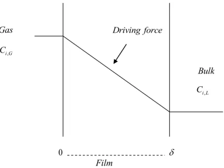
Figure 3-2. Diagram depicting the transfer of gas from the gas-phase to the bulk liquid……..……34
x
Figure 3-3. Plot of Power number against Reynolds number (Couper et al., 2005)……..…………45
CHAPTER 4 Figure 4-1. Glass flask system………48
Figure 4-2. The experimental stainless steel rig excluding the cold traps………..50
Figure 4-3. Vapour exit line leaving the reactor……….50
Figure 4-4. Ethylene-glycol bath containing the first two traps……….51
Figure 4-5. Ethanol bath containing the difluorodimethyl ether cold trap……….52
Figure 4-6. Difluorodimethyl ether cold trap……….52
Figure 4-7. Reactor vessel with the PVDF gasket………..53
Figure 4-8. Vertical insulated stainless steel condenser shown without insulation...……….54
Figure 4-9. The experimental glass rig excluding the cold traps…..………..……54
Figure 4-10. Process and instrumentation diagram for the selective production of difluorodimethyl ether in a stainless steel semi-batch reactor...………...56
Figure 4-11. Process and instrumentation diagram for the selective production of difluorodimethyl ether in a glass reactor …...57
Figure 4-12. The valve panel: front view and back view………...59
Figure 4-13. Reactor apparatus………...60
Figure 4-14. Schematic of temperature control system………..62
Figure 4-15. Solenoid valves and vacuum degassing manifold……….62
Figure 4-16. Ethanol bath used for the degassing process……….63
Figure 4-17. Process and instrumentation diagram of the kinetic study for the selective production of difluorodimethyl ether from R-22 in a jacketed glass reactor…...64
Figure 4-18. Hamilton Visiferm DO ARC probe in reactor..……….65
xi
Figure 4-19. Rig for sensor lag measurements………...66
Figure 4-20. Calibration chart for the R-22 rotameter………68
Figure 4-21. Calibration chart for the N2 rotameter………69
Figure 4-22. WIKA CTH 6500 display with thermo stated oil bath………..69
Figure 4-23. Calibration of the temperature sensor………71
Figure 4-24. Temperature uncertainty plot……….71
Figure 4-25. A typical chromatogram showing the component peaks………...73
Figure 4-26. The critical components of a spectrophotometer (Fritz and Schenk, 1979)…………..77
Figure 4-27. Calibration of standards for the spectrophotometric analysis of chlorides………80
Figure 4-28. Box-Behnken design with design points of radius 2 from the centre of the cube…..84
Figure 4-29. Box-Behnken design at the experimental conditions………85
CHAPTER 5 Figure 5-1. The effect of initial base concentration on the yield of difluorodimethyl ether at 298.15 K. Reactor system used; , glass; , stainless steel; , stainless steel with water………87
Figure 5-2. The effect of initial base concentration on the conversion of R-22 at 298.15 K. Reactor system used; , glass; , stainless steel; , stainless steel with water………..87
Figure 5-3. The effect of initial base concentration on the selectivity of difluorodimethyl ether at 298.15 K. Reactor system used; , glass; , stainless steel; , stainless steel with water…………88
Figure 5-4. Effect of temperature on the yield of difluorodimethyl ether at 2 mol·dm-3. Reactor system used; , glass; , stainless steel……….89
Figure 5-5. The effect of temperature on the conversion of R-22 at 2 mol·dm-3. Reactor system used; , glass; , stainless steel……….90
xii
Figure 5-6. Effect of temperature on the selectivity of difluorodimethyl ether at 2 mol·dm-3. Reactor
system used; , glass; , stainless steel……….90
Figure 5-7: A comparison of difluorodimethyl ether yield for experiments performed with water, , and without water, , at 298.15 K in the stainless steel reactor……….92
Figure 5-8: A comparison of R-22 conversion for experiments performed with water, , and without water, , at 298.15 K in the stainless steel reactor………...92
Figure 5-9. Hypothetical plot of the concentration path of the individual salts in the reactor...100
Figure 5-10a. Parity plot for sodium chloride concentration at 283 K...102
Figure 5-10b. Parity plot for total salt mass at 283 K...102
Figure 5-11a. Parity plot for sodium chloride concentration at 293 K...102
Figure 5-11b. Parity plot for total salt mass at 293 K...102
Figure 5-12a. Parity plot for sodium chloride concentration at 303 K...102
Figure 5-12b. Parity plot for total salt mass at 303 K...102
Figure 5-13. Concentration of NaCl produced vs. time, at 283.15 K with an initial NaOH concentration of 2 mol·dm-3 and an R-22 partial pressure of 40 kPa (•, experimental; ---, model)...104
Figure 5-14. Concentration of NaCl produced vs. time, at 283.15 K with an initial NaOH concentration of 2 mol·dm-3 and an R-22 partial pressure of 60 kPa (•, experimental; ---, model)...104
Figure 5-15. Concentration of NaCl produced vs. time, at 283.15 K with an initial NaOH concentration of 2.5 mol·dm-3 and an R-22 partial pressure of 50 kPa (•, experimental; ---, model)...104
Figure 5-16. Concentration of NaCl produced vs. time, at 283.15 K with an initial NaOH concentration of 1.5 mol·dm-3 and an R-22 partial pressure of 50 kPa (•, experimental; ---, model)...104
xiii
Figure 5-17. Concentration of NaCl produced vs. time, at 293.15 K with an initial NaOH concentration of 1.5 mol·dm-3 and an R-22 partial pressure of 40 kPa (•, experimental; ---, model)...105 Figure 5-18. Concentration of NaCl produced vs. time, at 293.15 K with an initial NaOH concentration of 2.5 mol·dm-3 and an R-22 partial pressure of 40 kPa (•, experimental; ---, model)...105 Figure 5-19. Concentration of NaCl produced vs. time, at 293.15 K with an initial NaOH concentration of 2.5 mol·dm-3 and an R-22 partial pressure of 60 kPa (•, experimental; ---, model)...105 Figure 5-20. Concentration of NaCl produced vs. time, at 293.15 K with an initial NaOH concentration of 1.5 mol·dm-3 and an R-22 partial pressure of 60 kPa (•, experimental; ---, model)...105 Figure 5-21. Concentration of NaCl produced vs. time, at 303.15 K with an initial NaOH concentration of 2 mol·dm-3 and an R-22 partial pressure of 40 kPa (•, experimental; ---, model)...106 Figure 5-22. Concentration of NaCl produced vs. time, at 303.15 K with an initial NaOH concentration of 2 mol·dm-3 and an R-22 partial pressure of 60 kPa (•, experimental; ---, model)...106 Figure 5-23. Concentration of NaCl produced vs. time, at 303.15 K with an initial NaOH concentration of 1.5 mol·dm-3 and an R-22 partial pressure of 50 kPa (•, experimental; ---, model)...106 Figure 5-24. Total salt mass vs. time at 283.15 K with an initial NaOH concentration of 2 mol·dm-3 and an R-22 partial pressure of 40 kPa (•, experimental; ---, model)...107 Figure 5-25. Total salt mass vs. time at 283.15 K with an initial NaOH concentration of 2 mol·dm-3 and an R-22 partial pressure of 60 kPa (•, experimental; ---, model)...107 Figure 5-26. Total salt mass vs. time at 283.15 K with an initial NaOH concentration of 2.5 mol·dm-
3 and an R-22 partial pressure of 50 kPa (•, experimental; ---, model)...107 Figure 5-27. Total salt mass vs. time at 283.15 K with an initial NaOH concentration of 1.5 mol·dm-
3 and an R-22 partial pressure of 50 kPa (•, experimental; ---, model)...107
xiv
Figure 5-28. Total salt mass vs. time at 293.15 K with an initial NaOH concentration of 1.5 mol·dm-
3 and an R-22 partial pressure of 40 kPa (•, experimental; ---, model)...108
Figure 5-29. Total salt mass vs. time at 293.15 K with an initial NaOH concentration of 2.5 mol·dm- 3 and an R-22 partial pressure of 40 kPa (•, experimental; ---, model)...108
Figure 5-30. Total salt mass vs. time at 293.15 K with an initial NaOH concentration of 2.5 mol·dm- 3 and an R-22 partial pressure of 60 kPa (•, experimental; ---, model)...108
Figure 5-31. Total salt mass vs. time at 293.15 K with an initial NaOH concentration of 1.5 mol·dm- 3 and an R-22 partial pressure of 60 kPa (•, experimental; ---, model)...108
Figure 5-32. Total salt mass vs. time at 303.15 K with an initial NaOH concentration of 2 mol·dm-3 and an R-22 partial pressure of 40 kPa (•, experimental; ---, model)...109
Figure 5-33. Total salt mass vs. time at 303.15 K with an initial NaOH concentration of 2 mol·dm-3 and an R-22 partial pressure of 60 kPa (•, experimental; ---, model)...109
Figure 5-34. Total salt mass vs. time at 303.15 K with an initial NaOH concentration of 1.5 mol·dm- 3 and an R-22 partial pressure of 50 kPa (•, experimental; ---, model)...109
Figure 5-35a. Arrhenius plot for reaction 1...110
Figure 5-35b. Arrhenius plot for reaction 2...111
Figure 5-36a. Parity plot of sodium chloride concentration for total fitting...113
Figure 5-36b. Parity plot of total salt mass for total fitting...113
Figure 5-37. Concentration of NaCl produced vs. time for total fitting, at 283.15 K with an initial NaOH concentration of 2 mol·dm-3 and an R-22 partial pressure of 40 kPa (•, experimental; ---, model)...114
Figure 5-38. Concentration of NaCl produced vs. time for total fitting, at 283.15 K with an initial NaOH concentration of 2 mol·dm-3 and an R-22 partial pressure of 60 kPa (•, experimental; ---, model)...114
Figure 5-39. Concentration of NaCl produced vs. time for total fitting, at 283.15 K with an initial NaOH concentration of 2.5 mol·dm-3 and an R-22 partial pressure of 50 kPa (•, experimental; ---, model)...114
xv
Figure 5-40. Concentration of NaCl produced vs. time for total fitting, at 283.15 K with an initial NaOH concentration of 1.5 mol·dm-3 and an R-22 partial pressure of 50 kPa (•, experimental; ---, model)...114 Figure 5-41. Concentration of NaCl produced vs. time for total fitting, at 293.15 K with an initial NaOH concentration of 1.5 mol·dm-3 and an R-22 partial pressure of 40 kPa (•, experimental; ---, model)...115 Figure 5-42. Concentration of NaCl produced vs. time for total fitting, at 293.15 K with an initial NaOH concentration of 2.5 mol·dm-3 and an R-22 partial pressure of 40 kPa (•, experimental; ---, model)...115 Figure 5-43. Concentration of NaCl produced vs. time for total fitting, at 293.15 K with an initial NaOH concentration of 2.5 mol·dm-3 and an R-22 partial pressure of 60 kPa (•, experimental; ---, model)...115 Figure 5-44. Concentration of NaCl produced vs. time for total fitting, at 293.15 K with an initial NaOH concentration of 1.5 mol·dm-3 and an R-22 partial pressure of 60 kPa (•, experimental; ---, model)...115 Figure 5-45. Concentration of NaCl produced vs. time for total fitting, at 303.15 K with an initial NaOH concentration of 2 mol·dm-3 and an R-22 partial pressure of 40 kPa (•, experimental; ---, model)...116 Figure 5-46. Concentration of NaCl produced vs. time for total fitting, at 303.15 K with an initial NaOH concentration of 2 mol·dm-3 and an R-22 partial pressure of 60 kPa (•, experimental; ---, model)...116 Figure 5-47. Concentration of NaCl produced vs. time for total fitting, at 303.15 K with an initial NaOH concentration of 1.5 mol·dm-3 and an R-22 partial pressure of 50 kPa (•, experimental; ---, model)...116 Figure 5-48. Total salt mass vs. time for total fitting at 283.15 K with an initial NaOH concentration of 2 mol·dm-3 and an R-22 partial pressure of 40 kPa (•, experimental; ---, model)...117 Figure 5-49. Total salt mass vs. time for total fitting at 283.15 K with an initial NaOH concentration of 2 mol·dm-3 and an R-22 partial pressure of 60 kPa (•, experimental; ---, model)...117
xvi
Figure 5-50. Total salt mass vs. time for total fitting at 283.15 K with an initial NaOH concentration of 2.5 mol·dm-3 and an R-22 partial pressure of 50 kPa (•, experimental; ---, model)...117 Figure 5-51. Total salt mass vs. time for total fitting at 283.15 K with an initial NaOH concentration of 1.5 mol·dm-3 and an R-22 partial pressure of 50 kPa (•, experimental; ---, model)...117 Figure 5-52. Total salt mass vs. time for total fitting at 293.15 K with an initial NaOH concentration of 1.5 mol·dm-3 and an R-22 partial pressure of 40 kPa (•, experimental; ---, model)...118 Figure 5-53. Total salt mass vs. time for total fitting at 293.15 K with an initial NaOH concentration of 2.5 mol·dm-3 and an R-22 partial pressure of 40 kPa (•, experimental; ---, model)...118 Figure 5-54. Total salt mass vs. time for total fitting at 293.15 K with an initial NaOH concentration of 2.5 mol·dm-3 and an R-22 partial pressure of 60 kPa (•, experimental; ---, model)...118 Figure 5-55. Total salt mass vs. time for total fitting at 293.15 K with an initial NaOH concentration of 1.5 mol·dm-3 and an R-22 partial pressure of 60 kPa (•, experimental; ---, model)...118 Figure 5-56. Total salt mass vs. time for total fitting at 303.15 K with an initial NaOH concentration of 2 mol·dm-3 and an R-22 partial pressure of 40 kPa (•, experimental; ---, model)...119 Figure 5-57. Total salt mass vs. time for total fitting at 303.15 K with an initial NaOH concentration of 2 mol·dm-3 and an R-22 partial pressure of 60 kPa (•, experimental; ---, model)...119 Figure 5-58. Total salt mass vs. time for total fitting at 303.15 K with an initial NaOH concentration of 1.5 mol·dm-3 and an R-22 partial pressure of 50 kPa (•, experimental; ---, model)...119 Figure 5-59. Simulated concentration vs. time profile for sodium methoxide at 293.15 K with an initial NaOH concentration of 2 mol·dm-3 and an R-22 partial pressure of 50 kPa...120 Figure 5-60. A profile of the simulated cumulative superficial salt concentration in the liquid vs.
time at 293.15 K with an initial NaOH concentration of 2 mol·dm-3 and an R-22 partial pressure of
50 kPa (-, NaCl; -, NaF)……….121
APPENDIX F
Figure F-1. Sensor lag plot: repeat measurement I………...……148 Figure F-2. Sensor lag plot: repeat measurement II……….…………148
xvii
Figure F-3. Sensor lag plot: repeat measurement III………149
Figure F-4. kLa measurements for oxygen at 283.15 K: measurement I………..149
Figure F-5. kLa measurements for oxygen at 283.15 K: measurement II……….150
Figure F-6. kLa measurements for oxygen at 293.15 K: measurement I………..150
Figure F-7. kLa measurements for oxygen at 293.15 K: measurement II……….151
Figure F-8. kLa measurements for oxygen at 293.15 K: measurement III………...151
Figure F-9. kLa measurements for oxygen at 303.15 K: measurement I………..152
Figure F-10. kLa measurements for oxygen at 303.15 K: measurement II………...152
Figure F-11. kLa measurements for oxygen at 303.15 K: measurement III……….153
xviii List of Tables
CHAPTER 2
Table 2-1. Examples of refrigerants that are CFCs, HCFCs and HFCs (Whitman et al., 2005)……..5
Table 2-2. Comparison of physical characteristics between carbon and various halogens (Kirsch, 2004)……….6
Table 2-3.Ozone depleting potential and atmospheric lifetime of popular refrigerants (Tiwary and Collins, 2010)………...8
Table 2-4. Atmospheric lifetimes and global warming potentials of HFEs (Tsai W., 2005)………...9
Table 2-5. Physical and thermo physical properties of a good refrigerant (Sapali, 2009; Mohanraj et al., 2009).………...11
Table 2-6. Chemical properties of a good refrigerant (Sapali, 2009; Mohanraj et al., 2009)……....11
Table 2-7. Thermodynamic properties of a good refrigerant (Sapali,2009; Mohanraj et al., 2009)..12
Table 2-8. Properties of an ideal refrigerant (Sapali, 2009)....………...13
Table 2-9. Fragmentation details for difluorodimethyl ether and trimethyl orthoformate (Satoh et al., 1998)………...17
Table 2-10. Ion-selective electrodes available for chloride analysis………..21
Table 2-11. Spectrophotometric methods in literature for chloride analysis……….22
Table 2-12. Titration methods in literature for fluoride analysis………...25
Table 2-13. Ion selective electrode for fluoride analysis………26
Table 2-14. Spectrophotometric methods in literature for fluoride analysis………..27
xix CHAPTER 3
Table 3-1. Final derived reactions with the respective heats of reaction………...29
Table 3-2. Concentration-based Henry’s law constants at the experimental temperatures…………36
Table 3-3. Solubilities of the two product salts that are formed in methanol……….41
CHAPTER 4 Table 4-1. PID tuning parameters………...……70
Table 4-2. Operating conditions of the Shimadzu GC 2014………..……72
Table 4-3. Sensor lag measurements………..76
Table 4-4. Overall mass transfer coefficients measured for oxygen and R-22………..77
Table 4-5. Coded variables for the Box-Behnken design………...84
CHAPTER 5 Table 5-1. Shimadzu QP 2010 G.C.M.S operating conditions...89
Table 5-2. Performance factors for experiments undertaken with water in the stainless steel reactor at 298.15 K...91
Table 5-3. Results of the Box-Behnken experimental design for kinetic data generation………….93
Table 5-4. Parameters obtained from the isothermal fitting procedure………110
Table 5-5. Arrhenius parameters for reaction 1 and reaction 2 (isothermal fitting)……….111
Table 5-6. Arrhenius parameters for reaction 1 and reaction 2 (total fitting) using Ksalt= 0.712 and m= 22.43……….112
xx APPENDIX B
Table B-1. Experimental vapour-liquid equilibrium data for R-22 (a) and methanol (b)
(Takenouchi et al., 2001)………...136 Table B-2. Physical properties of liquid methanol and R-22 gas………...136 Table B-3. Two forms of the Henry’s law constant for the R-22/methanol system at the temperatures of interest………137
APPENDIX C
Table C-1. Peak areas obtained from gas chromatograms for the residual gas………139 Table C-2. Peak areas obtained from the gas chromatograph for the cold trap gas………….……141
APPENDIX D
Table D-1. Properties of methanol and dimensions of impeller………...…144 Table D-2. Reactor vessel dimensions……….144 Table D-3. Data obtained from Nishiumi et al. (2003)………...………...145 Table D-4. Limiting ionic conductance and molar conductance for CH3ONa in methanol at 298.15 K………...146 Table D-5. Limiting ionic conductances at 303.15 K for CH3ONa in methanol……….146
APPENDIX E
Table E.1. List of chemical data for materials used……….147
xxi
NOMENCLATURE
A Absorbance %
A Pre-exponential factor -
A c Surface area of coil m2
A i Peak area m2
C Concentration mol·dm-3
C* Oxygen saturated concentration mol·dm-3
C0 Initial concentration at zero time mol·dm-3
C p Heat capacity J·mol-1·K-1
d b Average bubble size m
d c Coil tube diameter m
d imp Impeller diameter m
d t Tank diameter m
D Diffusivity m2·s-1
E a Activation energy kJ·mol-1
E A Enhancement factor -
F Faraday’s constant C·mol-1
g Gravitational acceleration m2·s-1
Ha Hatta number -
h i Heat transfer coefficient W·m-2·K-1
Hcc Concentration-based Henry’s law constant -
H pc Henry’s law constant or partition coefficient dm3·kPa·mol-1
H f Enthalpy of formation kJ·mol-1
H r Enthalpy of reaction kJ·mol-1
H s Enthalpy of solution kJ·mol-1
K Sechenov coefficient -
k 1 Reaction rate constant for reaction 1 (dm3·mol-1)2·min-1 k 2 Reaction rate constant for reaction 2 (dm3·mol-1)·min-1
k l Thermal conductivity W·m-1·K-1
k L Liquid-side mass transfer coefficient m·min-1
k a L Volumetric mass transfer coefficient min-1
k M Mass transfer coefficient min-1
probe
k Sensor lag constant min-1
xxii
L Length of coil m
m Mixing parameter
m Mass flow rate of coolant kg·s-1
M Molecular mass g·mol-1
n Molar flow rate mol·min-1
n Valence of cation/anion -
N Impeller speed rps
P Power W
P i Partial pressure Pa
Q Volumetric flow rate m3·min-1
Q r heat rate W
r Rate of reaction mol·dm-3·min-1
R Universal gas constant J·mol-1·K-1
Ri Net rate of change for component i mol·dm-3·min-1
S Selectivity %
t Time min
T Transmittance (Section 4.3.) %
T Temperature K
U Overall heat transfer coefficient W·m-2·K-1
V Volume dm3
V m Molar volume of mixture dm3·mol-1
V s Superficial gas velocity m·s-1
x Mole fraction -
X Conversion %
Y Yield %
Greek letters
Film thickness m
Surface tension N·m-1
Pi -
Density kg·m-3
Gas-holdup (dimensionless) -
i2
Variance of data point i -
Solvent viscosity Pa·s
Solvent association parameter -
Limiting ionic conductances (A·cm-2)(V·cm-1)(g-
equiv·cm-3)
Stoichiometric coefficient -
xxiii Subscripts and Superscripts
b Bulk phase
G Gas
L Liquid
m Order of reactant 1 n Order of reactant 2 LM Logarithmic mean
1
CHAPTER 1 INTRODUCTION
1.1. Background and motivation
Chlorodifluoromethane (R-22) has been widely used as an industrial and domestic refrigerant since the 1950s (Calm, 2008). The hydro-chlorofluorocarbon (HCFC) molecule exhibits acute stability with an atmospheric lifetime of 15.3 years (Tiwary and Collins, 2010). The chlorine atom in a molecule of R-22 gas reacts with ozone in the stratosphere, causing the destruction of the ozone layer (Halimic et al., 2003).
Figure 1-1a). A molecule of R-22 Figure 1-1b). A molecule of difluorodimethyl ether
The potential of R-22 gas to deplete the ozone layer has deemed it unsuitable for use as a general refrigerant. Hydrofluoroethers (HFEs) represent potential alternatives to HCFCs, possessing physical and thermodynamical properties that are suitable for refrigeration applications. HFEs are less stable than R-22 and do not contribute to ozone depletion as they are unlikely to reach the stratosphere. A typical example of this new generation of refrigerants, difluorodimethyl ether, can be conveniently produced via the reaction of R-22 and methanol in the presence of sodium hydroxide. This synthesis also provides a means of converting current reserves of R-22 into a useful product (Nishiumi and Kato, 2003).
The synthesis of difluorodimethyl ether from R-22 and methanol in the presence of sodium hydroxide has formed the basis of numerous studies such as that of Lee et al. (2001) and Nishiumi and Kato (2003). Lee et al. (2001) investigated the effect of reaction temperature, concentration of
2
base and the chemical nature of the base on the yield of difluorodimethyl ether. The authors found that lower reaction temperatures and base concentrations favoured the formation of difluorodimethyl ether (Lee et al., 2001). They also found that the use of alkali metal carbonates resulted in superior difluorodimethyl ether yields in comparison to the alkali metal hydroxides;
however, the synthesis required reaction temperatures well above the normal boiling point of methanol and high pressures (Lee et al., 2001). Kato and Nishiumi (2003) studied the aforementioned reaction at 303 K. A stationary-state reaction model was developed, which included the mass transfer characteristics of the system. An overall volumetric mass transfer coefficient and rate constant were reported only at 303 K. There is a lack of credible kinetic data in the literature for this reaction system over a wider range of operating conditions. Therefore, the collection and analysis of rate data for the reaction of R-22 and methanol in the presence of sodium hydroxide were carried out using a stirred semi-batch gas-liquid reactor. A Box-Behnken experimental design, comprising 12 experiments, was used for the generation of the kinetic data. Reaction temperature, partial pressure of R-22 and initial sodium hydroxide concentration were varied simultaneously according to the design.
1.2. Objectives
The overall objective of the project was to develop a kinetic model for the reaction of R-22 and methanol in the presence of sodium hydroxide and to identify the kinetic parameters. In order to achieve this objective, a number of different tasks had to be carried out. Firstly, the effect of reaction conditions on the product distribution had to be investigated using a statistical experimental design. Apart from yielding important information regarding the most preferable operating range, this stage also served to generate kinetic data for the identification procedures. Next an appropriate mathematical model had to be developed for the three-phase reactor, taking into account gas-liquid interfacial mass transfer as well as reactions in the bulk liquid. Thereafter, the rate data generated using the statistical experimental design had to be critically evaluated and the kinetic parameters of the gas-liquid reactions had to be determined in the temperature range of 283.15 -303.15 K.
1.3. Thesis outline
This chapter has served as a brief introduction to the reaction system considered in this investigation. It has also identified the main objectives associated with this project. Chapter two
3
provides further detail on fluoroorganic compounds, the chemistry of ozone destruction and the use of fluorinated ethers as replacement refrigerants. In chapter three, the development of the kinetic model and the reactor modeling are presented. The chapter also provides a theoretical understanding of the concepts to be discussed in chapters four and five. Chapter four discusses the equipment used together with the materials and methods that were required. The presentation and discussion of the results is dealt with in chapter five. The conclusions drawn from the research and recommendations for future work are given in chapter six.
4
CHAPTER 2
LITERATURE REVIEW
2.1. Fluoroorganic compounds: characteristics
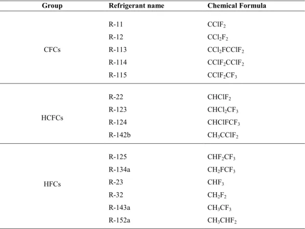
The skeletal backbone of most fluorochemical refrigerants is methane and ethane. The elements of concern in the two molecules are carbon (C) and hydrogen (H). Chlorination and/or fluorination of either molecule generate refrigerant groups such as chlorofluorocarbons (CFCs), hydro- chlorofluorocarbons (HCFCs), hydro-fluorocarbons (HFCs) and perfluorocarbons (PFCs) (Whitman et al., 2005). Table 2-1 lists examples of each refrigerant group (Whitman et al., 2005).
Figure 2-1. Methane molecule
Figure 2-2. Ethane molecule
5
Table 2-1. Examples of refrigerants that are CFCs, HCFCs and HFCs (Whitman et al., 2005)
Group Refrigerant name Chemical Formula
CFCs
R-11 CClF2
R-12 CCl2F2
R-113 CCl2FCClF2
R-114 CClF2CClF2
R-115 CClF2CF3
HCFCs
R-22 CHClF2
R-123 CHCl2CF3
R-124 CHClFCF3
R-142b CH3CClF2
HFCs
R-125 CHF2CF3
R-134a CH2FCF3
R-23 CHF3
R-32 CH2F2
R-143a CH3CF3
R-152a CH3CHF2
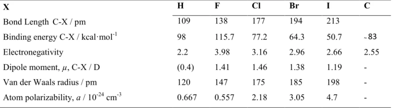
The above-mentioned refrigerants are fluoroorganic compounds. The bond between the carbon and fluorine atom in fluoroorganic compounds is radically stable (Kirsch, 2004). The stability can be attributed to the overlap of the fluorine 2s and 2p orbitals and the respective carbon orbital; as well as the fluorine substituent that blocks the central carbon atom (Kirsch, 2004). The bond is also physically characteristic of a high polarity and electronegativity (Kirsch, 2004). A comparison of physical characteristics between carbon and various halogens is listed in Table 2-2 (Kirsch, 2004).
6
Table 2-2. Comparison of physical characteristics between carbon and various halogens (Kirsch, 2004)
X
Bond Length C-X / pm Binding energy C-X / kcal·mol-1 Electronegativity
Dipole moment, µ, C-X / D Van der Waals radius / pm Atom polarizability, a / 10-24 cm-3
H F Cl Br I C
109 138 177 194 213
98 115.7 77.2 64.3 50.7 ~ 83
2.2 3.98 3.16 2.96 2.66 2.55
(0.4) 1.41 1.46 1.38 1.19 -
120 147 175 185 198 -
0.667 0.557 2.18 3.05 4.7 -
2.2. Chemistry of ozone destruction
Ozone (O3) is produced by the interaction of sunlight with oxygen (Parker and Morrissey, 2003). It is a rare molecular structure of oxygen, shielding the earth from the ultraviolet radiation generated by the sun. Approximately 90% of the ozone is found in the stratosphere (Parker and Morrissey, 2003). The stratosphere is that part of the atmosphere in which chemical reactions, mainly due to the presence of chlorine radicals, take place (Mohanraj et al., 2009). It stretches from 10 km above the surface of the earth to approximately 50 km beyond (Mohanraj et al., 2009). In this region, a relatively high concentration of ozone can be found.
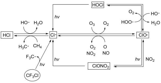
Chlorofluorocarbons, perfluorocarbons and halofluorocarbons, to list a few, cannot be degraded below the stratosphere because of their acute chemical stability. As a result the compounds enter the stratosphere. Chlorofluorocarbons for example undergo photolytic dissociation in the stratosphere despite showing high stability in the low level atmosphere (Kirsch, 2004). The carbon-chlorine bond terminates releasing the chlorine radical. The chlorine radical is then free to react with ozone (O3) to form oxygen (O2) and chlorooxide radicals (ClO•). The chlorooxide radical can be converted back into chlorine by reaction with nitrous oxide (NO), nitric oxide (NO2), atomic oxygen (O) or hydroperoxy radicals (HOO•). The chlorine radical may also react with methane present in the stratosphere to form HCl, which in turn may react with hydroxyl radicals to re-form the chlorine radical. Figure 2-3 describes graphically the catalytic process by which the ozone is depleted. The catalytic process described was summarized from the literature (Kirsch, 2004).
7
Figure 2-3. Catalytic process instrumental in the depletion of the ozone layer (Kirsch, 2004)
2.2.1. Ozone depleting potential
Ozone depleting potential (ODP) is a relative measure of the magnitude of degradation to the ozone layer by a substance capable of depleting the ozone layer (a gas) (Halimic et al., 2009). The base reference used is trichlorofluoromethane (R-11) with an ODP of 1.0 (Halimic et al., 2009). The ODP of R-22 relative to R-11 is 0.05 (Tiwary and Collins, 2010). Table 2-3 lists the ODP of popular refrigerants (hydrocarbons) and their lifespan in the stratosphere. Of this list, the least harmful refrigerants are HFC-125, HFC-134a, HFC-143a and HFC-152a with no ODP. Carbon tetrachloride is the most harmful refrigerant with an ODP of 1.1. HFEs possess a zero ODP due to the absence of the chlorine atom in these refrigerants.
8
Table 2-3.Ozone depleting potential and atmospheric lifetime of popular refrigerants (Tiwary and Collins, 2010)
Halocarbon ODP Lifetime / years
CFC-11 1.00 (by definition) 60
12 0.9 120
113 0.85 90
114 0.6 200
115 0.37 400
HCFC-22 0.05 15.3
123 0.017 1.6
124 0.02 6.6
HFC-125 0 28.1
134a 0 15.5
HCFC-141b 0.095 7.8
142b 0.05 19.1
HFC-143a 0 41
152a 0 1.7
Carbon tetrachloride (CCl4) 1.1 50
Methyl chloroform (CH3CCl3) 0.14 6.3
2.2.2. Global Warming Potential
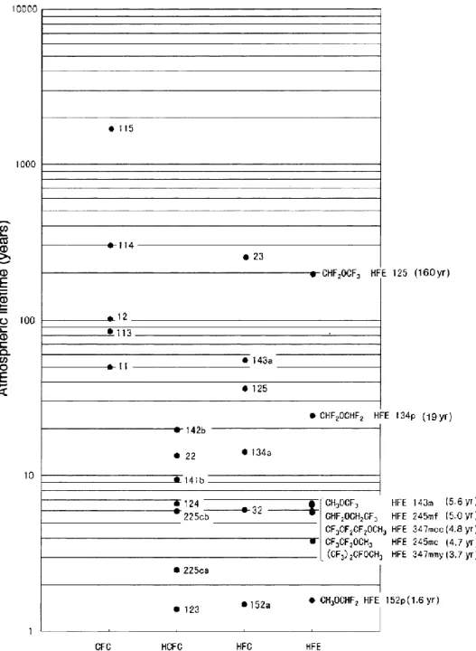
Global warming potential (GWP) is defined as „the ratio of calculated steady state net infrared flux change forcing at the troposphere for each unit mass of any halocarbon emitted relative to the same for CFC-11‟ (Banks et al., 2000). Anthropogenic substances emitted into the environment cause the temperature of the earth‟s surface to increase. Such a phenomenon is referred to as global warming (Tsai W., 2005). A comparison of the GWP of HFEs listed in Table 2-4 to the GWP of common refrigerants depicted graphically in Figure 2-4 indicates a relatively greater GWP for CFCs and HCFCs. Figure 2-4 illustrates a GWP range between 2000 and 12000 for CFCs and HCFCs whereas Table 2-4 lists a range between 39 and 15600 for HFEs.
9
Table 2-4. Atmospheric lifetimes and global warming potentials of HFEs (Tsai W., 2005)
The atmospheric lifetime of CFCs, HCFCs, HFCs and HFEs is shown graphically in Figure 2-4 (Sekiya and Misaki, 2000).
10
Figure 2-4.Atmospheric lifetimes of CFCs, HCFCs, HFCs and HFEs (Sekiya and Misaki, 2000)
11
2.3. Properties and Characteristics of refrigerants
A substance, be it a fluoroorganic compound or a natural chemical (such as carbon dioxide), may be categorized as a refrigerant if it exhibits the necessary properties that define a refrigerant.
Thermodynamic, physical and chemical properties are all important attributes of a good refrigerant.
2.3.1. Physical Properties
Table 2-5 lists the physical and thermo physical properties that are desirable of a good refrigerant (Sapali, 2009; Mohanraj et al., 2009).
Table 2-5. Physical and thermo physical properties of a good refrigerant (Sapali, 2009; Mohanraj et al., 2009)
Physical Property Characteristic
Specific volume Low
Viscosity Low
Thermal conductivity High
Dielectric strength High
2.3.2. Chemical Properties
Chemical properties are important to ensure that refrigeration systems operate safely. The properties listed in Table 2-6 are summarized from the literature (Sapali, 2009; Mohanraj et al., 2009).
Table 2-6. Chemical properties of a good refrigerant (Sapali, 2009; Mohanraj et al., 2009)
Chemical Property Characteristic
Toxicity Non-toxic
Flammability Low, must not be inflammable
Flashpoint < 294.35 K
Stability Unreactive with metals,
Must be able to withstand the effect of pressure and temperature without decomposition
Corrosiveness Non-corrosive
Leak detection (smell) Must be easy to detect a leak
12
2.3.3. Thermodynamic properties
Table 2-7 lists the thermodynamic properties characteristic of a good refrigerant (Sapali, 2009;
Mohanraj et al., 2009).
Table 2-7. Thermodynamic properties of a good refrigerant (Sapali, 2009; Mohanraj et al., 2009)
Thermodynamic Property Characteristic
Latent heat of evaporation High
Boiling point Low
Freezing point Lower than system temperature
Evaporating pressure Slightly greater than atmospheric
Condensing pressure Low
Critical temperature and pressure Must be greater than condensing temperature
A high latent heat of evaporation is preferable because a lower power requirement implies that less refrigerant can be used to produce greater cooling effects (Sapali, 2009). A freezing point temperature that is lower than evaporating temperature will prevent freezing of the refrigerant (Sapali, 2009; Mohanraj et al., 2009). A low condensing pressure will simplify construction and reduce leakages (Sapali, 2009).
2.3.4. An ideal refrigerant
Table 2-8 lists properties that are characteristic of ideal refrigerants; summarized from the literature (Sapali, 2009).
13
Table 2-8. Properties of an ideal refrigerant (Sapali, 2009)
Property Description Specification
Thermodynamic
ODP Zero
GWP Zero
Latent heat of evaporation High
Critical pressure High
Critical temperature High
Condensing pressure High
Evaporating pressure High
Chemical
Toxicity Non-toxic
Flammability Non-flammable
Corrosiveness Non-corrosive
Miscibility with oil Low
Physical Leak detection Easy
Cost and availability Cheap and available
2.4. Substitution of chlorine containing fluoroorganic compounds with HFEs
Hydrofluoroethers are regarded as the new generation of eco-friendly refrigerants. Their potential as candidate alternatives to CFCs, HCFCs and PFCs was investigated by Sekiya and Misaki (2000) as part of the “development of new refrigerants, blowing agents and cleaning solvents for effective use of energy” initiative. As a part of their investigation, 150 fluorinated ethers were evaluated as alternatives to blowing agents, refrigerants and cleaning solvents. This review is concerned specifically with fluorinated ethers as refrigerant replacements.
It is imperative that the profile of the fluorinated ether not lose the integrity of the physical, chemical and thermodynamic properties of refrigerants. Yet, at the same time, the fluorinated ethers should not pose a threat to the environment unlike the CFC counterparts (Sekiya and Misaki, 2000).
14
Since the fluorine atom in CFCs provides the basis for good properties and fluorine does not contribute to ozone depletion, it is the fundamental key to an alternative (Sekiya and Misaki, 2000).
Fluorinated compounds exhibit all the properties of a suitable refrigerant. Sekiya and Misaki (2000) theorized that in order for compounds to not pose an environmental threat, the compounds must decompose at a faster rate than CFCs. The authors proposed that this is attainable by the introduction of a hydrogen atom into the molecule and the elimination of chloride and bromide ions.
The researchers only considered tests on fluorinated ethers with short life spans (between 1 and 5 years). Physical properties such as density, specific heat, surface tension, thermal stability and flammability were investigated (Sekiya and Misaki, 2000). The toxicity of the fluorinated ethers is negligible, and, of the various fluorinated ethers investigated, none has possessed a boiling point close to R-22. However, three fluorinated ethers were discovered that possessed properties similar to R-11 and R-114. These are regarded as suitable alternatives.
2.5. Dechlorination of R-22 with methanol 2.5.1. Reaction schemes
Difluorodimethyl ether can be formed via the reaction of R-22 with methanol in the presence of sodium hydroxide. The actual mechanism of dechlorination has been investigated by a number of authors (Hine and Porter, 1957; Lee et al., 2001; Satoh et al., 1998). The extraction of a halide ion from a halogen containing compound occurs via one of two mechanisms: an SN2 mechanism or a dehydrohalogenation mechanism. The objective of the research undertaken by Hine and Porter (1957) was to confirm which of the mechanisms applied to chlorodifluoromethane (R-22), and thereby introduce a scheme for the reactions.
The mechanism of the SN2 reaction is drawn in Figure 2-5. A polar bond exists between carbon and the halogen (Bruice, 2004). The halogen is more electronegative than the carbon. As a result, the halogen and the carbon have partially negative and positive charges, respectively (Bruice, 2004).
A nucleophile (OH-) is attracted to the electrophile (C) forming a new bond. Simultaneously, the carbon-halogen bond is broken heterolytically (Bruice, 2004).
15
Figure 2-5. Substitution reaction (Bruice, 2004)
Elimination reactions, in particular, the dehydrohalogenation mechanism, involve the simultaneous removal of a halogen (Cl, F, I, Br) and a proton (H) from the alkyl halide (Bruice, 2004). The mechanism for the α-dehydrohalogenation mechanism is drawn in Figure 2-6.
Figure 2-6. Elimination reaction (Bruice, 2004)
In α-eliminations (dehydrohalogenation), the proton and the halide are positioned on the same carbon atom. A nucleophile (OH-) removes a proton (H), subsequently forming a carbanion. The halogen is then removed from the carbanion, forming a carbene (Bruice, 2004).
Hine and Porter (1957) initially suspected the reaction between R-22 and methanol, in the presence of sodium hydroxide, to occur via the SN2 mechanism. The authors conducted a test to determine the rate at which the methoxide ion (CH3O-) reacts. The approximate rate constant was found experimentally to be 4.5×10⁻⁶ dm3·mol-1·s-1 at 308.15 K. However, α-fluorine decreases SN2 reactivity and therefore the authors anticipated a slower reaction (Hine and Porter, 1957). The authors discounted the plausibility of the SN2 mechanism and considered instead, the α- dehydrohalogenation to form difluoromethylene (:CF2), followed by the reaction to form the only two organic products: difluorodimethyl ether and trimethyl orthoformate. Difluoromethylene formation was considered to be a major reaction. It is an intermediate that reacts further with methanol to produce difluorodimethyl ether and trimethyl orthoformate. The reaction scheme suggested by Hine and Porter (1957) is drawn in Figure 2-7.
16
CHClF2 + CH3ONa :CF2 + CH3OH + NaCl
:CF2 CH3OCHF2
(CH3O)3CH
CH3OH
2CH3ONa, -2NaF
:C(OCH3)2 CH3OH
Figure 2-7. Reaction scheme 1 (Hine and Porter, 1957)
Satoh et al. (1998) proposed that trimethyl orthoformate was not produced from difluoromethylene.
Rather, it was formed consecutively with difluorodimethyl ether. Figure 2-8 shows the reaction scheme suggested by Satoh et al. (1998). The authors reported that the removal of difluorodimethyl ether, upon formation, will lower the formation of trimethyl orthoformate.
CHClF2 + CH3ONa CH3OCHF2 + NaCl CH3OCHF2 + 2CH3ONa (CH3O)3CH + 2NaF
Figure 2-8. Reaction scheme 2 (Satoh et al., 1998)
Lee et al. (2001) investigated this reaction system to confirm the validity of either proposed mechanism. Difluorodimethyl ether was reacted with sodium methoxide (sodium hydroxide in methanol) for 2 hours at 298.15 K. The reaction produced a trace quantity of trimethyl orthoformate, thus strongly proving the mechanism by Satoh et al. (1998) implausible and the scheme by Hine and Porter (1957) plausible. The reaction as shown by Hine and Porter (1957) and rewritten by Lee et al. (2001) is drawn in Figure 2-9.
(2-1) (2-2)
17
CHClF2 + CH3ONa :CF2 + CH3OH + NaCl
:CF2 CH3OCHF2
(CH3O)3CH
CH3OH
2CH3ONa, -2NaF
:C(OCH3)2 CH3OH
Figure 2-9. Reaction scheme 3 (Lee et al., 2001)
2.5.2. Experimental studies of the production of difluorodimethyl ether from R-22
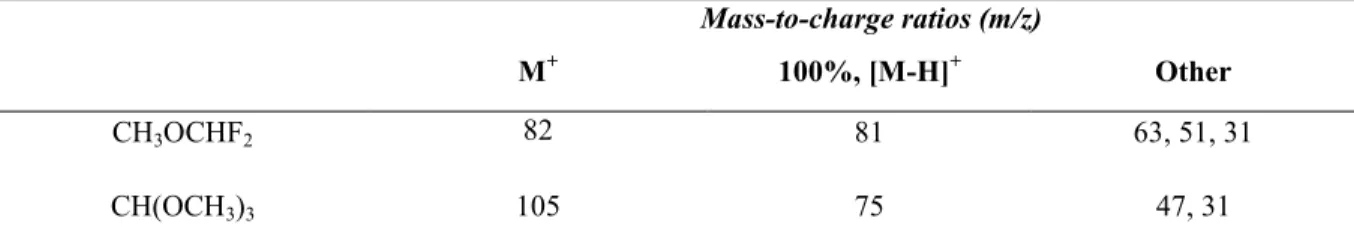
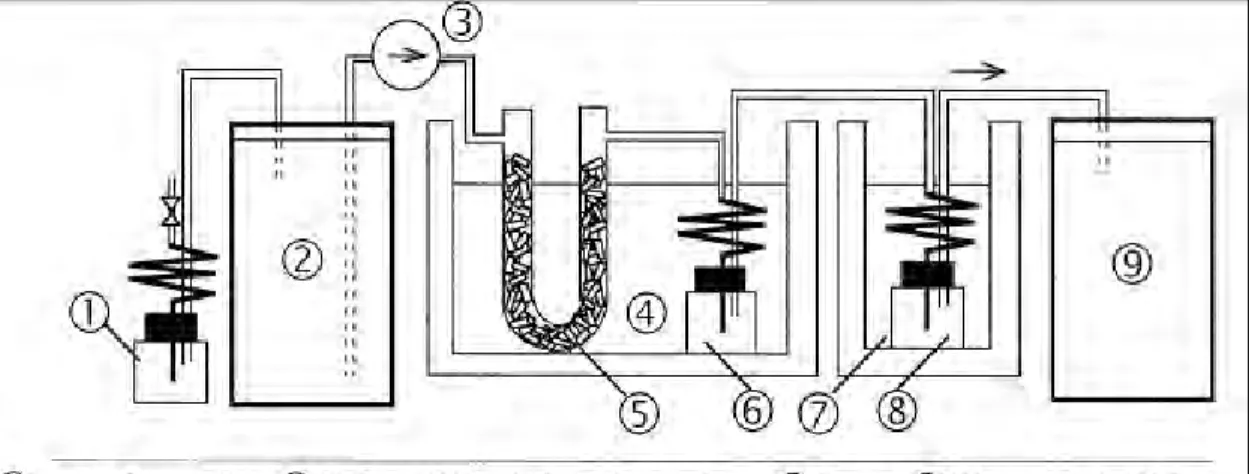
Satoh et al. (1998) measured the vapour pressure of difluorodimethyl ether, once synthesized from the reaction between R-22 and methanol. Vapour pressures are a good indication of the suitability of a compound as a refrigerant (Satoh et al., 1998). Two sets of apparatus were used for the synthesis of difluorodimethyl ether and the vapour pressure measurements. The initial apparatus was a circulating type system. R-22 emanating from the product stream was constantly recycled through the circuit. Figure 2-10 depicts the circulating system as an excerpt from the original paper.A yield of 70% difluorodimethyl ether was obtained. A by-product was discovered and found to be trimethyl orthoformate. This was confirmed by injection of product and by-product into the GCMS.
The analysis provided fragmentation information on the products. The fragmentations of the products are listed in Table 2-9. The authors used the fragmentation spectra to identify the two products. In particular, the M+ or molecular ion peak gave an indication of the relative formula mass (molecular mass) of the compounds. Other molecular fragments, including the most abundant peak ([M-H]+), were used to piece together the molecular structure.
Table 2-9. Fragmentation details for difluorodimethyl ether and trimethyl orthoformate (Satoh et al., 1998)
Mass-to-charge ratios (m/z)
M+ 100%, [M-H]+ Other
CH3OCHF2 82 81 63, 51, 31
CH(OCH3)3 105 75 47, 31
18
Figure 2-10. Circulating type system (Satoh et al., 1998)
Satoh et al. (1998) reported that the removal of difluorodimethyl ether, immediately after formation would reduce the formation of trimethyl orthoformate. A flow system was therefore commissioned by the authors. Figure 2-11 depicts the excerpt of the apparatus from Satoh et al. (1998). R-22 gas was injected by the vapour pressure, into the reactor containing a solution of sodium hydroxide and methanol, at a rate of 1 dm3·min-1 (Satoh et al., 1998). The reactor was maintained at 273.15 K in a water bath. The product gas was then cooled as it entered two consecutive cold traps submerged in an ethylene glycol bath at 268.15 K. The first cold trap contained molecular sieve 5A to remove methanol. The second cold trap separated the by-product from the product gas stream. The difluorodimethyl ether gas was liquefied in the third cold trap at 238.15 K.
Figure 2-11. Flow type system (Satoh et al., 1998)
19
The difluorodimethyl ether liquid collected was passed through three distillation steps to obtain a difluorodimethyl ether purity of 94.5% and a yield of 63%. The distillation process shown in Figure 2-12 is an excerpt taken from Satoh et al. (1998). The 2-propanol bath was set at 253.15, 258.15 and 263.15 K for the three steps of distillation.
Figure 2-12. Distillation apparatus for the flow type system (Satoh et al., 1998)
The vapour pressure measurements undertaken by the authors involved two sets of apparatus. The first apparatus was valid for the temperature range 260 to 290 K in a water bath. The second apparatus was applicable for temperatures greater than 290 K in an air bath. Temperature was measured with a platinum-resistant thermometer. Pressure was measured with a Bourdon gauge.
Between 266 and 393 K, no difluorodimethyl ether decomposition was noticed.
Lee et al. (2001) suggested the use of alkali metal carbonates as a more efficient base system to suppress the formation of trimethyl orthoformate and increase the yield of difluorodimethyl ether.
K2CO3, Na2CO3 and Li2CO3 were reported as possible replacements to sodium hydroxide in methanol. The effect of reaction parameters on the formation of trimethyl orthoformate was investigated prior to analyzing the performance of the mentioned bases. The authors observed an increase in difluorodimethyl ether yield with temperature at constant base concentration. A decrease of difluorodimethyl ether yield with base concentration was observed at constant temperature. The author‟s findings show that trimethyl orthoformate formation cannot be suppressed by changes to reaction temperature or sodium methoxide concentration.
20
Nishiumi and Kato (2003) studied the effect of salt concentration on the dechlorination of R-22 and suggested that the accumulation of sodium chloride in the reactor resulted in less efficient mixing of the NaOH/methanol solution (Nishiumi and Kato, 2003). They noted that the white precipitate of sodium chloride was visible due to the low solubility of sodium chloride in methanol. They postulated that the accumulation of sodium chloride precipitate and the inhibitory effect on mixing reduced the mass transfer rate. A simple model of the reaction system was developed which ignored the production of sodium fluoride. The effect of sodium chloride on the rate of mass transfer was accounted for by the addition of a correction to the mass transfer coefficient. This correction factor was a function of the total salt concentration. It appeared to be satisfactory since the mass transfer coefficient is a function of the intensity of mixing as inferred from the presence of impeller speed in many established mass transfer correlations.
2.6. Analytical methods
2.6.1. Determination of chloride ion concentration
The Mohr method is a classical procedure in the analysis of chloride ion concentration (Murthy, 1995). It is described as an argentometric titration in which silver nitrate is used to precipitate silver chloride. The end-point is detected by the formation of a reddish-brown precipitate, silver chromate, formed by the reaction of an excess of silver ions with chromate (Radojević, 2006). Unfortunately there is no experimental evidence that there is no interference from fluoride ions that may be present in the solution.
The mercurimetric method developed in 1933 by Dubsky used diphenylcarbohydrazine as an indicator for mercuric nitrate titration (Zall et al., 1956). To determine the concentration of the chloride ion by colorimetric means, Barney (1957) suggested the reaction of chloride with mercuric chlorinilate to liberate the acid chlorinilate ion. The downfall of this method is the unavailability of commercial mercuric chlorinilate. It is also an expensive procedure to prepare mercuric chlorinilate.
Ion selective electrodes can also be used for the determination of chloride ion concentration. Table 2-10 lists the available ion selective electrodes, with which chloride ions can be analyzed efficiently and