Using the 2011 South African population census, we provide income and multidimensional poverty and inequality estimates at the municipal level. Our results show that both income and multidimensional poverty and inequality vary significantly between municipalities in South Africa. In this paper we examine the spatial distribution of poverty and inequality in contemporary South Africa.
In this paper, we provide estimates of poverty and inequality at the municipal level. Using the two approaches together provides a better picture of the spatial distribution of well-being across South Africa. In this paper, we examine the spatial distribution of poverty and inequality, and the relationship between poverty, inequality and other factors in South Africa.
Todes and Turok (2017) provide a detailed review of the various spatial initiatives and policies implemented in the past in South Africa. We use income data from the 2011 South African Census to estimate income poverty and inequality at the local municipality level.
Exploratory spatial data analysis
Patterns of inequality and poverty across municipalities
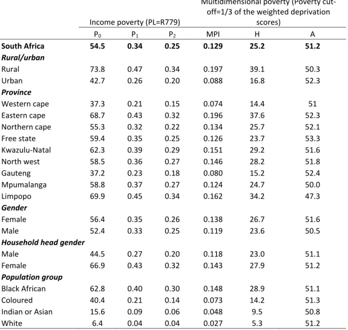
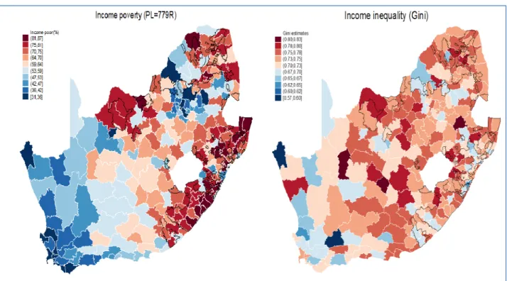
11 Among the largest metropolitan cities (Ekurhuleni, City of Johannesburg, City of Tshwane, eThekwini, Mangaung, Nelson Mandela Bay, City of Cape Town and Buffalo City), the income poverty rate is relatively lower in the city of Cape Town. , the City of Tshwane and the City of Johannesburg (about 35%-36%), while the figure is about 52%-54% in the City of Buffalo and Nelson Mandela Bay. Estimates of the Gini coefficient show that the level of income inequality is at least 0.57 in all municipalities. The level of income poverty in these municipalities ranges from 63% in Renosterberg to 72% in Abaqulusi.
Koofiishiin walqixxummaa galii Gini bulchiinsa magaalota torba keessatti gadi aanaa yoo ta’u lakkoofsi kun Laingsburg, Richtersveld, Vulamehlo, Bergrivier, Cederberg, Nqutu, Hessequa gidduutti garaagarummaa qaba). Walqixxummaan galii Nqututti 0.65, Maphumulotti 0.68 hanga Mbizana fi Tulluu Ngquzaatti 0.77 ture. Tilmaamni MPI bulchiinsa magaalota dureeyyii kurnan (Swartland, Drakenstein, Saldanha Bay, Bergrivier, Magaalaa Johaannesbarg, Langeberg, Witzenberg, Magaalaa Keep Taawun, Stellenbosch, Mossel Bay, Magaalaa Tshwane) fi hiyyeeyyii hiyyeeyyii kurnan keessaa 0.058 fi 0.074 gidduutti argama .
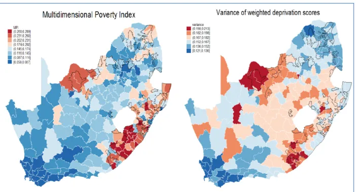
The proportion of people considered multidimensionally poor is 14% and less the rich ten municipalities, the figure varies between 50%-54% in the poorest ten municipalities. Among the largest cities, inequalities in deprivation are relatively lower in the City of Cape Town and Johannesburg, while the figure is higher in Buffalo and Mangaung City. We also find that inequalities in multidimensional deprivation in municipalities seem higher in poor municipalities. These results are consistent with a recent finding by Sartorius and Sartorius (2016), which shows that although there are large differences in the provision of services between richer and poorer districts, within districts inequality is higher in both richer urban areas and poorer ones rural areas.
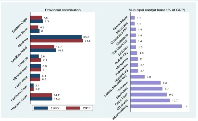
The figure shows large differences in the level of economic activities across municipalities in South Africa. For example, GDP per inhabitant in the richest municipality close to 100% of GDP per inhabitant of the poorest. The figure shows that the 10 richest municipalities include (Tlokwe City Council, Overstrand, Bela-Bela, Mookgopong, Steve Tshwete, Rustenburg, Modimolle, Knysna, Govan Mbeki and the town of Matlosana).
The City of Johannesburg and eThekwini are ranked 18th and 19th respectively in terms of per capita, while Cape Town is ranked 37th.
Spatial autocorrelation
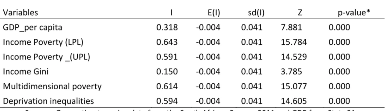
These results suggest that there is significant and positive spatial dependence in the distribution of regional development. Source: Own estimates based on data from the South African Census, 2011 and GDP from Stats SA. Although the global Moran's I suggests a significant positive spatial autocorrelation, the approach does not tell us whether regional heterogeneities in development patterns exist.
For this purpose, we use local Moran's I statistics, which allow us to determine whether high or low values are spatially clustered (Anselin, 1995). A positive value for the local Moran I statistic indicates that a given municipality has neighboring municipalities with similarly high or low poverty or inequality scores (detecting clustering), while a negative value indicates that a municipality has neighboring municipalities with different poverty or inequality scores (detecting divergence). . The z-score of the local Moran's index I and its p-value are used to test whether clustering features or outliers are statistically significant.
We find that there are significant clusters of high-income poverty and multidimensional measures of poverty (hotspots) mainly around KwaZulu-Natal and the Eastern Cape provinces. In contrast, the cold spots are found in municipalities located in the Western Cape (for all measures) as well as for poverty around the clustered areas of Gauteng. In the case of multidimensional estimates, we find some areas with clusters of low-high poverty estimates. Three municipalities with relatively lower multidimensional scores (Greater Kokstad, The Msunduzi, eThekwini) are surrounded by municipalities with higher levels of poverty.
Estimation results for the correlates of poverty
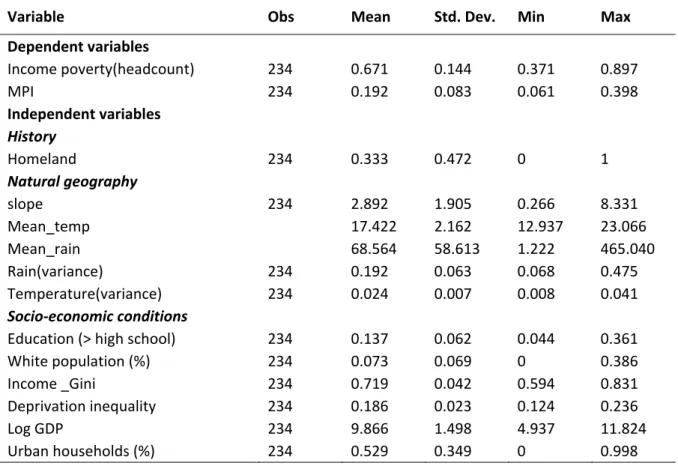
The parameter ρ represents the magnitude of the spatial autoregressive process on poverty; namely, how poverty rates between neighboring regions mutually influence each other. In addition to the spatial autoregressive process in the dependent variable, the SDM records spillovers from the effects of explanatory variables from neighboring municipalities. With the aim of disentangling the complex nature of spatial poverty, we use three categories of independent variables: historical, geographical and socio-economic factors to take into account the fact that, in the case of South Africa, poverty and inequality are shaped by the country's geography and history.
As a baseline estimate, we run OLS regression without spatial terms which we only present in Table 2B in the appendix because it is technically inferior to our spatial models. The positive and significant correlation of the former home country dummy in both estimates shows the influence of historical factors on current poverty. The estimation results in Tables 3 and 4 are based on the use of the row-normalized binary spatial weight matrix (both connectivity and inverse-distance spatial weights).8 In both the SAR and SDM model estimations, we include all the variables used in the OLS . model.
The corresponding estimates based on the inverse distance spatial weights are given in Table 3B and Table 4B in the Appendix. Note: The results presented were obtained using the inverse distance spatial weights in the Appendix. In econometric terms, the existence of this autocorrelation may have caused biases in the OLS estimates of β in Table 2B of the Appendix.
According to the form of Direct, Indirect and Total effects, in SDM the indirect effect increases due to In the case of SDM, with an inverse-distance spatial weight and with the interaction term, the coefficient on the proportion of white population is significant with a negative sign, and income inequality is positive and marginally significant. The indirect effect coefficients measuring spatial spillovers are larger in SDM than in SAR.
We can see that the effects of each of the variables are systematically smaller in the spatial models than in the OLS case. This is why the estimation results of the home country coefficient in SDM (with inverse distance spatial weight matrix) suggest an insignificant coefficient that then becomes significant after adding the interaction term of home country with the share of the population that has a higher education. Our spatial models prove very useful in unpacking the large impact of the homeland dummy variable on poverty that we see in the non-spatial estimations of the municipality-level data as well as in our previous mapping.
Conclusions
Our results show that once these spillovers are taken into account, being part of a home country is not correlated with current income poverty rates. Rather, these rates are mainly explained by education, urban ratio and the average rain volume. It is now possible to compare the coefficients of the direct effects and the OLS estimates in table 2.
In particular, the coefficients of home country dummy become smaller and even statistically insignificant in some spatial model estimations. Some of this effect is due to the fact that those living within these apartheid borders are still particularly prone to the socio-economic hardships that drive contemporary poverty. 26 The spatial models allow for the estimation of a total effect, which includes both direct intra-
Now poverty rates are mainly explained by local education levels, urban proportions and the average rainfall volume. Most notably, the large negative coefficient attributed by OLS to living within a historic homeland area is greatly reduced and even not statistically significant in some spatial models. However, when interactions between this historical geographic variable and contemporary socioeconomic hardship are included, homeland becomes statistically significant again.
This makes the important point that while, across the county, it is these socio-economic deprivations that are particularly important in explaining contemporary income poverty, those still living in these areas of the homeland remain particularly disadvantaged in terms of these deprivations. First, our analysis of poverty and inequality, and the relationship between the two, is based on a single census and, as such, is a static analysis. Change in most variables including inequality and GDP per capita takes time and, as such, these static correlations are no substitute for long-term estimates of how changes in these variables affect poverty and inequality.
These include the scale of public spending, local level capacity and efficiency of local level spending, and even corruption.
Using indicators of multiple deprivation to demonstrate the spatial legacy of apartheid in South Africa. Economic geography and growth in Africa: The case of sub-national convergence and divergence in South Africa. Service delivery inequality in South African municipal areas: A new way of accounting for inter-jurisdictional differences.
Appendix A: Multidimensional Poverty and Inequality Estimates
Children aged <7 years - not deprived of schooling, and children aged 7 and 8 years - not deprived if they are currently attending school (even if they have not completed any schooling).
Appendix B: Tables and Figures