Bruun Rule Equation Source:(Bruun, 1988)
Landsat radiometric calibration equation
MNDWI equation
Kappa coefficient equation
DSAS Shoreline Uncertainty Equation
Best Fit Linear Equation
DSAS Standard Error Equation
Shoreline Position Index equation
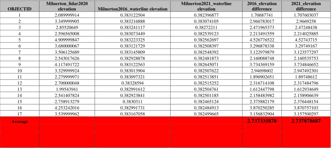
Pixel Height Mean Difference
BACKGROUND
The presence of beaches greatly increases Cape Town's tourism potential, but sea level rise threatens accessibility along coastal roads and railways and attractions such as tidal pools (Dube et al., 2021). The risk of sea level rise was compounded by the fact that real estate development doubled between 1980 and 2007 near the high water mark and on reclaimed land (Colenbrander et al., 2014).
PROBLEM STATEMENT
While progress has been made in understanding South Africa's coastlines, coastal erosion remains a growing problem. Global directions such as the Sustainable Development Goals (SDGs) can only be specifically addressed in the local context of South Africa.
SCOPE AND JUSTIFICATION OF STUDY
South Africa has a predominantly sandy coastline and this is the basis of this research (Fourie et al., 2015). Although there are various aspects of using GIS in coastal management, the general expectation of this study is to use satellite imagery to analyze coastal erosion.
RESEARCH QUESTIONS
AIM & OBJECTIVES
Research questions 3: What specific geoprocessing techniques within optical and microwave remote sensing can be combined as suitable for shoreline extraction and beach profiling, respectively, towards a complete analysis of coastal erosion.
RESEARCH SIGNIFICANCE AND PRACTICAL APPLICATIONS
SUMMARY
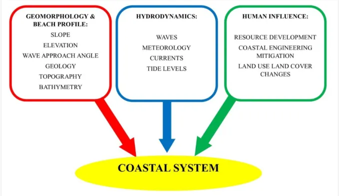
As already said, remote sensing is versatile, but its applicability lies in first understanding the components of the phenomenon of interest. The first section addresses the major influences on coastal environments, while the second highlights the compatibility of remote sensing as a tool to achieve the above objectives.
BEACH PROFILE MORPHODYNAMICS
- SEDIMENT TRANSPORT MECHANISMS
- SHORELINE TYPES
- TIDES
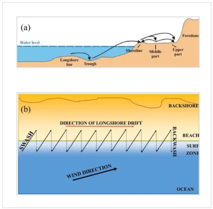
Longshore currents move sand in a sawtooth-like motion, as depicted in Figure 3 (Almar et al., 2019). Tides are the oscillating response of the oceans to the gravitational effects of the sun and moon, as well as the rotational force of the Earth (Bird & Coasts, 1984; Searson & Brundrit, 1995).
APPLICATION OF REMOTE SENSING AND GIS IN COASTAL STUDIES
- THE THEORY OF REMOTE SENSING
- SENSOR DESIGN
- SENSOR PLATFORM SELECTION
- COASTAL OBSERVATION INDICATORS
Certain wavelengths can be absorbed, reflected or transmitted based on the nature of the surface (Deronde et al., 2008). It is one of the most widely used indices for vegetation monitoring that includes the NIR and Red bands (Tingzon et al., 2020).

CURRENT LITERATURE ON COASTAL REMOTE SENSING
- APPLICATION OF OPTICAL SENSORS IN COASTAL EROSION MONITORING
- APPLICATION OF LIDAR TECHNOLOGY IN COASTAL MONTORING
- APPLICATION OF RADAR SATELLITES IN COASTAL MONITORING
- MULTI-DIMENSIONAL DATA FUSION FOR SHORELINE MEASUREMENT
Edge detection or waterline extraction for radar images can be problematic due to the woodpecker noise (Niedermeier et al., 2005). Amaro et al.(2014) designed a labor intensive method that incorporated both moderate and high resolution satellite imagery, as well as a Post Processing Kinematic (PPK) GPS survey (Amaro et al., 2014).
SUMMARY
The need for sensors with specific spectral resolutions based on the spectral signatures of coastal areas has been of particular concern to researchers. There have been several efforts to perform a comparative analysis of remote sensing techniques based on different project objectives (Boak & Turner, 2005; Cracknell, 2010; Hamylton, 2017).
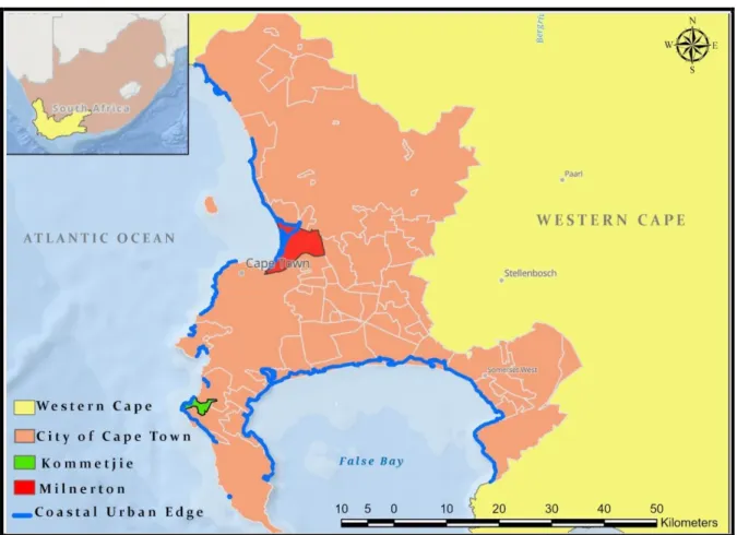
CASE STUDY: THE CAPE TOWN COASTLINE
It is now abundantly clear that the South African government recognizes the importance and threats to coastal areas (Colenbrander et al., 2014). Since then, it has guided tactics for spatial planning and sustainable development (Colenbrander et al., 2014).

STUDY SITES
The literature review responds that optical and microwave based remote sensing techniques can be applicable, optimal and achievable for both shoreline extraction and beach profiling approaches towards a comprehensive analysis of coastal erosion. The literature review has also communicated previous research that other researchers have conducted in identifying appropriate remote sensing methods for coastal erosion observations. The methodology formulated here builds on this previous research and is split into two to fully incorporate shoreline extraction and beach profiling approaches towards a complete analysis of coastal erosion.
The purpose of this chapter is to justify, detail and highlight the relevance of the chosen tools in relation to the specified goals and objectives.
VISUAL PROXY-BASED MEASUREMENT OF HISTORICAL SHORELINE MOVEMENT
- MATERIALS AND DATASETS
- FUNCTIONAL COASTAL INDICATORS
- SOFTWARE AND TOOLS
- LAND-SEA SEGMENTATION FROM OPTICAL SATELLITE DATA
- MULTITEMPORAL POST-CLASSIFICATION SHORELINE MOVEMENT MODELLING
Land cover change statistics were also recorded and are further discussed in section 5.2 of the results. The direction of the transects depends on the smoothing distance as shown in Figure 14. The positional accuracy of the coastlines is determined via the Coastline Position Index, while the uncertainty of the DSAS statistics is calculated via the End Point Rate (EPR) (Himmelstoss et al. al., 2018).
The statistical accuracy of the DSAS tool is based on both weighted (WSE) and linear (LSE) regression.
DATUM-BASED BEACH PROFILING METHODS
- MATERIALS AND DATASETS
- FUNCTIONAL COASTAL INDICATORS
- SOFTWARE AND TOOLS
- APPLICATION OF WATERLINE METHOD FOR ELEVATION MODELLING
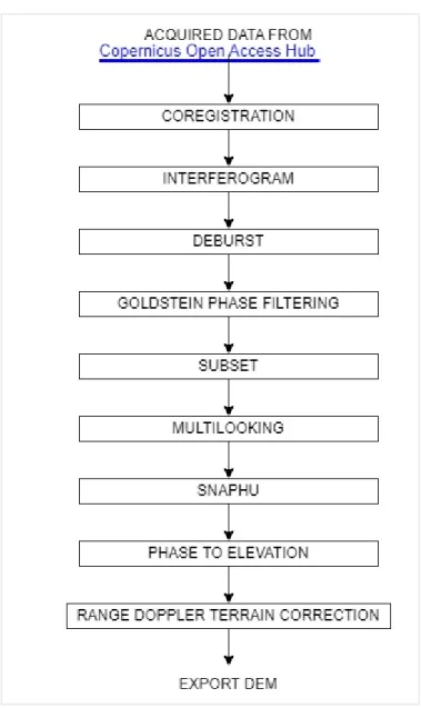
- DIFFERENTIAL INTERFEROMETRY (DInSAR)
- REAL TIME KINEMETIC (RTK) BEACH SURVEY
- DEM ACCURACY ASSESSMENT
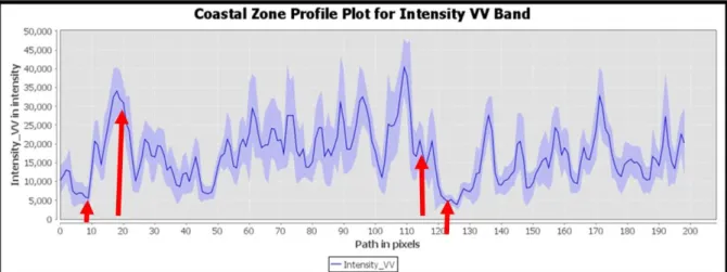
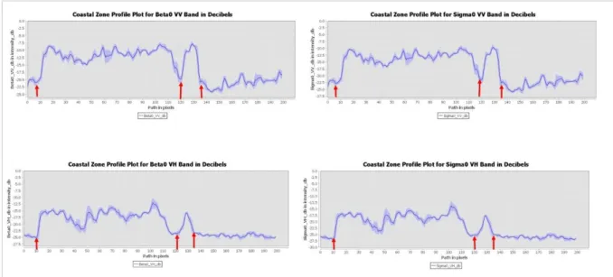
For the purposes of this study, the reference coastline was from the waterline boundary of the topographic survey described in the section below on page 81. Sentinel-1 coastlines obtained as described in 4.3.4.2 on page 76 were used as waterlines, while is tide gauge data was modeled and used to adjust the height of the water line. For proper use, the backscatter coefficient (σ o ) has been converted to decibels using a logarithmic function, as shown in Figure 17 (B) on page 75 below.
The initial visual state of the images was unintelligible and presented as a static filled image as shown in Figure 20 (a) on page 81.
SPECTRAL ANALYSIS
- MULTISPECTRAL BAND SELECTION FOR CLASSIFICATION
- RADAR BAND SELECTION FOR THRESHOLDING
The spectral properties of coastal areas and land cover changes as discussed in section 2.2.1.1 on page 18 are demonstrated here both statistically and visually. The graphs in Figure 30 below depict the combined effect of polarization and calibration on the ground cover response measured in decibels. It detects beach sand, rocks and ocean as a land cover leading to a false shoreline position.
Based on pixel changes, we can extract and quantify land use changes (Orlikova & Horak, 2019).

LAND COVER CHANGES
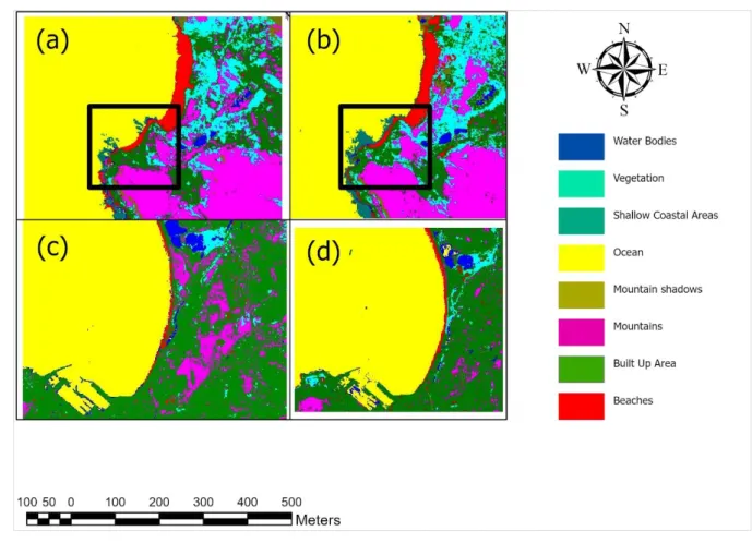
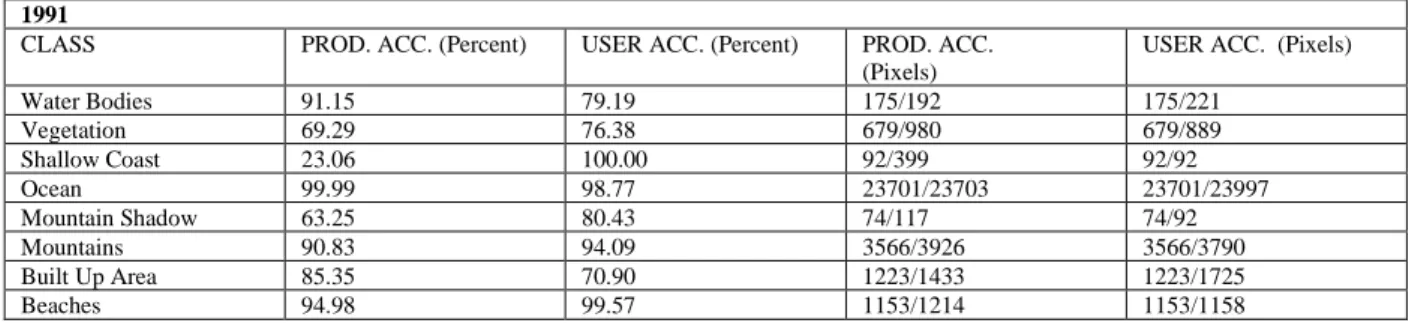
The images below show the result of the support vector classification over the study areas, as well as the changes in land cover condition 1991 and 2021 respectively, within the Milnerton and Kommetjie coastal areas. Although Milnerton Lagoon interacts with the ocean, it is still classified as an inland body of water. The overall ocean grade has experienced the least change overall, while Milnerton beach grade has increased by 38%, built-up areas by almost 13% and vegetation by 16%.
However, unlike Kommetjie, the Milnerton area has experienced a decline in shallow coastal areas.
CLASSIFICATION ACCURACY
Although it is visually noticeable that the coastal shallows have decreased in 2021 for Kommetjie, the beach areas (red land cover) appear to be thinning. It should be noted that the increase in beach surfaces is ultimately an increase in bare land, which is characterized by a spectral response of the land. Cape Town's landscape is also known for its hilly nature and the combination of cliff faces, vegetation and bare ground cover can lead to spectral confusion, which is why we use confusion matrices to determine how accurate are these classification schemes.
Manufacturer and user accuracy measurements can be found in APPENDIX A MANUFACTURER AND USER COVERAGE CLASSIFICATION MATRIX FOR 1991 AND 2021 on page 154.
CALCULATION AND ASSESSMENT OF SHORELINE CHANGE RATES
- SHORELINE POSITION CHANGE
- SHORELINE CHANGE ENVELOPE (SCE)
- NET SHORELINE MOVEMENT
- END POINT RATE
- STATISTICAL UNCERTAINTY
The drivers and implications of the statistics derived here are discussed under section 6.1 on page 136. Again, these erosion statistics coincide with the location of the lagoon mouth indicated by the red arrow in Figure 38 on page 106. There are sections of Milnerton Beach that have erosion rates of up to 6.23 m/yr.
Again, as indicated by a red arrow in Figure 40 on page 108, the highest EPR is observed at the mouth of Milnerton Lagoon.

FIELD OBSERVATIONS
Both beaches exhibit the same general biogenic sand profile with fine white beach sand mixed with fragmented shells as shown in Figure 43(a) above. The impact of aeolian erosion was also widespread on both beaches as depicted by the sand ripples in Figure 43(b). The bed was observed in Figure 44 (a) while the wave action is clearly exploiting their lines of weakness and the streaks were also observed in Figure 44 (b).
This was evidenced by the presence of a block nearly 20 feet long between the boulders, as shown in Figure 46, which many locals noted was displaced during high wave events.

BEACH PROFILE ANALYSIS
- TIDE MODELS
- ELEVATION MODELS
- RESOLUTION EFFECTS ON SHORELINE EXTRACTION
- BEACH PROFILE MORPHODYNAMICS CLASSIFICATION
Again, the curve along Kommetjie Beach has the lowest elevation and the same can be said along the opening of Milnerton Lagoon. Although the height values have been changed, the range of the values is still the same. As discussed in section 2.2 of the theory chapter on page 15, the sensitivity for detecting land cover varies according to the instrument used.
The Shoreline Position Index (I) equation as described in Section 4.2.6.3 on page 68 was used to determine the most accurate of the satellite sensors used in this study.
SHORLINE MOVEMENT ANALYSIS DISCUSSION
Hughes, supported the CSIR findings that the mouth of Milnerton Lagoon indicates a bimodal sediment transport system with northward sediment movement estimated at 100 000 m3/year. His study also concluded that there was a sediment deficit south of the mouth and that it was being actively eroded. It is not a question of adequacy and usability of DSAS, but more of data availability.
Hughes (1992) also echoed the same sense that erosion was less north of the lagoon opening than to the south with a sediment deficit.
BEACH PROFILING DISCUSSION
While a simple calculation of RMSE is acceptable when calculating individual DEM uncertainty, Salameh et al. (2020) points to the need for further evaluation of DEM differences (DOD). The main sources of sediment along the Atlantic coast are biogenic carbonate weathering, aeolian fine sand washed down through the Karbonkelberg Pass, and weathering of the Table Mountain Group bedrock. Two sections of the Cape Town coastline, Kommetjie and Milnerton along the Atlantic coast, were analyzed separately.
The combination of the MNDWI spectral index and SVM classification was found to be effective for coastline delineation.
RECOMMENDATIONS
Monitoring sediment dynamics along a sandy coastline by aerial hyperspectral remote sensing and LIDAR: a case study in Belgium. The use of the Normalized Difference Water Index (NDWI) in the demarcation of open water features. An assessment of the status quo, vulnerability and adaptation of the physical and socio-economic impacts of climate change in the Western Cape.
Geological mapping of the inner shelf along Cape Town's Atlantic coast, South Africa, Council for Geosciences.
SANHO Data Release Form
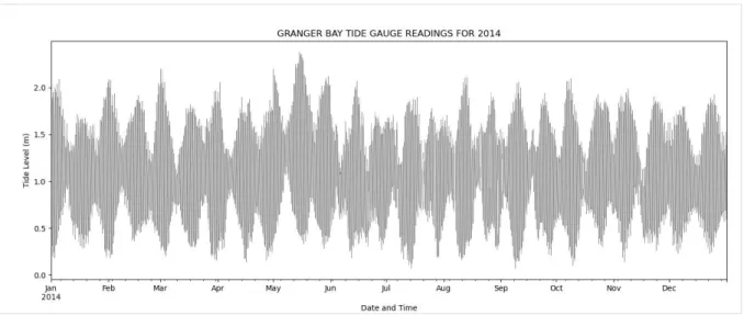
Harmonic Constituents For Granger Gay Tide Gauge In 2014
DT refers to date-time column, while SeaLevel is the actual tide from SANHO's tide gauge in Granger Bay. The prediction must be readjusted from the LAT hydrographic datum to Hartebeesthoek 94 land datum using the -0.98m offset my_prediction = tide.at(times).