KELLER-SEGEL CHEMOTAXIS EQUATIONS IN SCALE OF BANACH SPACES
By
David Shituula Ila-kutse Iiyambo
Submitted in fullment of the academic requirements for the degree of
Doctor of Philosophy in the School of
Mathematics, Statistics and Computer Science University of KwaZulu-Natal
Durban
December 2015
As the candidate's supervisor, I have/have not approved this thesis for submission.
Signed: . . . Name: Robert Willie (D. Sc. Maths. UCM-Spain) Date: . . . .
In this Thesis, we study the asymptotic and blow-up dynamics of Keller-Segel (KS) chemo- taxis equations in Lebesgue-Bochner spaces of underlying Banach spaces of either typeLp(Ω) or Bessel potential spaces (I −∆)−s2Lp(Ω) = Hs,p(Ω). The model equations involve the attraction or minimal, and the attraction-repulsion Keller-Segel (ARKS) chemotaxis equa- tions. The treatment yielded begins with a review of the semigroup action in Bessel potential spaces, and interpolation theory for their construction. In studying the well-posedness of the equations we establish a natural condition between the initial data spaces and spaces for the inhomogeneous terms of the equations, with which we prove the well-posedness of the dynamical system for an extended analytic semigroup in Banach spaces. The best con- stants of the function spaces embedding intoLρ-spaces yield, for either Banach xed point theorem, or global existence of solutions, no need for neither the time for a contraction mapping, nor initial data of the equations to be relatively small respectively. The global asymptotic dynamics of the system equations in time is captured in the limit set M × {0}, whereM=|Ω|L1(Ω) is of the spatial average solutions, and the approach to null states of the orthogonal to constant solutions is due to an a priori decay to zero of the drift chemical cues from that of the cells density. At several points in the work we have proved the existence of a priori uniform boundedness of the solutions to the equations in time and space, yielding via bootstrap arguments that the solutions are classical solutions. In blow-up dynamics, we obtain non-existence of solutions at the borderline space, independent of time, when the chemical coecient or dierence is above the Moser-Trudinger threshold value.
The contributions of the work, besides being at the interface of mathematical analysis and medical biology, lies in the fact that its mathematical analysis takes the most often used function spaces platform for the treatment of the equations a step further in frontier to the
ii
equations imply other non-linear terms of bio-physical relevance can be taken into account in modelling diversied complex phenomena that might be possibly more precise to describing the pathological situations arising in nature to the system of model equations. In blow-up dynamics of the equations our analysis does not limit the scientist concerned to the case of two dimensions corresponding to the particular case of the Hilbert space setting H1. The non-local elliptic equation reduction of the system equations still call for important other analysis to the topic in the general function space setting that insofar has been introduced, for instance the establishment of Palais-Smale condition, and Pohozaev inequality for non- existence of solutions at the borderline of the function spacesH2α,p(Ω). This last point we have resolved in the case of Hilbert spaces.
iii
I, David Shituula Ila-kutse Iiyambo, declare that
1. The research reported in this thesis, except where otherwise indicated, is my original research.
2. This thesis has not been submitted for any degree or examination at any other university.
3. This thesis does not contain other persons' writing, unless specically acknowledged as being sourced from other researchers. Where other written sources have been quoted, then:
(i) Their words have been re-written but the general information attributed to them has been referenced.
(ii) Where their exact words have been used, then their writing has been placed in italics and inside quotation marks, and referenced.
4. This thesis does not contain text, graphics or tables copied and pasted from the Internet, unless specically acknowledged, and the source being detailed in the thesis and in the References sections.
Signed:. . . .
iv
DETAILS OF CONTRIBUTION TO PUBLICATIONS that form part and/or include research presented in this thesis (include publications in preparation, submitted, in press and published and give details of contributions of each author to experimental work and writing of each publication)
Publication 1.
Iiyambo D., and Willie R., Semigroup and blow-up dynamics of attraction Keller-Segel chemotaxis equations in scale of Banach spaces., (Submitted to Analysis and Mathematical Physics on November 2015.
(There were regular meetings between myself and my supervisors to discuss research material for publications. The outline of the research papers and discussion of the signicance of the results were jointly done. The papers were mainly written by myself with some input from my supervisors.)
v
I declare that the contents of this dissertation are original except where due reference has been made. It has not been submitted before for any degree to any other institution.
David Shituula Ila-kutse Iiyambo June 10, 2016
vi
This Thesis is dedicated to the memory of my little brother Andreas.
The pain caused by your departure is only fractionally reduced by the
fond memories that we have of you.
Abstract ii
Table of Contents viii
Acknowledgements x
Introduction 1
0.1 Origin and Importance of the model in Biological Sciences and Mathematics . 1
0.2 Outline of the Thesis . . . 13
1 Preliminaries 16 1.1 Introduction . . . 16
1.2 Functional Setting . . . 16
1.3 Semigroups . . . 18
2 Interpolation theory 26 2.1 Interpolation theory background . . . 26
2.2 Real Interpolation . . . 34
2.3 Complex interpolation method . . . 36
2.4 Banach scales of Bessel potential spaces . . . 38
2.5 Banach scale spaces of positive operators . . . 40
3 Minimal KS Equation in Bessel Potential Spaces 53 3.1 Introduction . . . 53
3.2 Well-posedness of the System . . . 56
3.2.1 Proof of Theorem 3.2 . . . 60
3.3 Uniform Bounds of Solutions . . . 69
3.4 Blow-up Dynamics . . . 72
4 Attraction-Repulsion KS Equations in Scale of Hilbert Spaces 74 4.1 Introduction . . . 74
viii
4.2 Preliminaries . . . 77
4.3 Well-posedness of the system of equations . . . 80
4.4 Uniform bounds of solutions . . . 90
4.5 Equations in system coupled elliptic dierential operator . . . 101
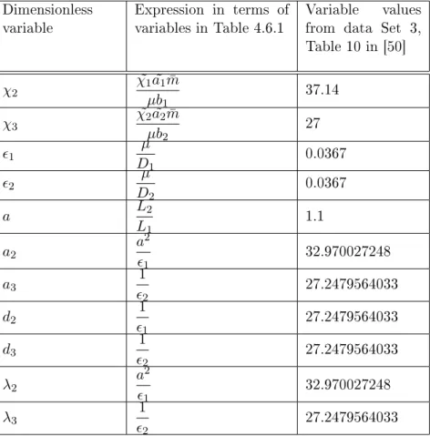
4.6 Numerical simulation . . . 107
4.6.1 Parameter values . . . 108
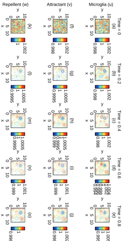
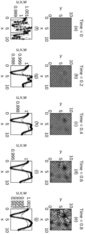
4.7 Discussion of results . . . 111
5 Minimal KS Equations Blow-up Analysis in Hilbert Spaces 116 5.1 Introduction . . . 116
5.2 Rescaling Solutions . . . 116
5.3 Global Existence of Blow-up solutions . . . 119
5.4 Blow-up . . . 125
5.5 Blow-up by the Concavity Method . . . 140
6 Attraction-Repulsion KS Equations in Scale of Banach Spaces 144 6.1 Introduction . . . 144
6.2 Preliminaries . . . 152
6.3 Well-posedness in Lσ( ˙I;Lp(Ω))spaces . . . 155
6.3.1 Boundedness in Ω×I˙ and asymptotic global dynamics . . . 160
6.4 Well -posedness in Epα spaces. . . 164
6.5 Blow-up dynamics . . . 175
Conclusion 177
Bibliography 178
Index 187
Firstly, I would like to thank the almighty God, for the gift of a healthy life and for making everything possible. Secondly, I would like to thank my supervisor, Dr. Robert Willie for agreeing to take me on, and subsequently, for his patience and encouragement throughout the course of this study. In the same vein, I would like to thank Professor J. Banasiak who refereed me to Dr. Willie during the time of my application for enrolment with the University of KwaZulu-Natal, School of Mathematics, Statistics and Computer Science. I would also like to register my appreciations to the three unanimous examiners who evaluated this thesis for the excellence in their detailed reviews that covered evaluations in all the chapters of this Thesis.
The Namibia Government Scholarship and Training Program (NGSTP) and the Uni- versity of Namibia Sta Development Program cannot be thanked enough for funding my studies.
My enormous gratitude goes to my Parents, Tate na Meme Iiyambo, for having done such a great job raising me, and for having sent me to school. As Robert Brault once said, A parent's love is whole no matter how many times it's divided". You are the best of them all.
My lovely wife Loini, you are my air. Thank you for taking a chance on me. I imagine it can't be easy being married to a man with as many aws as me. Winston Churchill said it best: My most brilliant achievement was my ability to be able to persuade my wife to marry me."
My best friend Komeine, thanks for being such a great trend-setter and an exemplary friend.
Everyone else who contributed either directly or indirectly towards this work, thank you and God bless.
Westville, Durban David S. I. Iiyambo
June 10, 2016
x
0.1 Origin and Importance of the model in Biological Sciences and Mathematics
Chemotaxis is a process characterised by the directed movement or orientation of organisms or cells, in response to the concentration gradient of an external chemical signal. The chemical signals can come from external sources, or they can be secreted by the organisms themselves. The situation where the chemical is produced by the organisms themselves leads to aggregation of organisms and to the formation of patterns.
In 1970, E.F. Keller and L.A. Segel [41] proposed a mathematical model describing this chemotactic aggregation of cellular slime molds Dictyostelium discoideum which move (in a domain Ω) preferentially towards relatively high concentrations of a chemical substance cAMP (cyclic adenosine monophosphate), produced by the amoebae themselves. Their derivation of the system of equation was, briey, as follows. Let u(x, t) denote the density of amoebae, v(x, t) := ψ2 denote the concentration of the chemical attractant. Then the four basic assumptions which underlie the derivations are (see [35, 41]):
1. The chemical attractant is produced per amoeba at a rate off(v).
2. There exists an extracellular enzyme that degrades the chemical attractant. The
1
concentration of the enzyme at time t in point x is denoted by w(x, t) := ψ3. This enzyme is produced by the amoebae at a rateg(v, w) per amoebae.
3. The chemical attractant and the enzyme react to form a complex of concentration z(x, t) :=ψ4, which dissociates into a free enzyme plus the degraded product.
4. v, w andz obey Fick's Law when diusing.
It then follows from the balance of the cell density in open bounded domain Ω ⊂ RN, with smooth boundary ∂Ω, during aggregation that
d dt
Z
Ω
u(x, t)dx= Z
Ω
Q(u)(x, t)dx− Z
∂Ω
J(u)(x, t)·~ndσ, (0.1) where Q(u)(x, t) represents the mass of amoeba created/dying per unit volume per unit time, while J(u)(x, t) = uχ3∇w−uχ2∇v− ∇u is the ux of amoeba mass. Note that the composition ofJ(u)(x, t)follows from using Fick's Law and Fourier's Law for the heat ow, and we have also taken a linear sensitivity function χ(s, t) =χ. If we neglect reproduction and death of the amoebae, thenQ(u)(x, t)≡0. Since the chemical attractantv, the enzyme w, and the complexz diuse, we get that
d dt
Z
Ω
ψ(t, x)dx= Z
Ω
Q(ψ)(x, t)dx− Z
∂Ω
J(ψ)(x, t)~ndσ, (0.2) whereJ(ψ) =−∇ψis the ux of either v, w or z, and Q(ψ)(x, t) is the chemical attractant or the enzyme or the complex produced per unit volume per unit time. One then uses the
divergence theorem on (0.1) and (0.2) to obtain the following system of equations
ut= ∆u−P3
i=2Div u(−1)iχi∇ψi
inΩ×(0, T), vt= ∆v−λ2vw+b2z+uf(v) inΩ×(0, T), wt= ∆w−λ2vw+b3z+ug(v, w) inΩ×(0, T), zt= ∆z+λ2vw−(b2+b3)z inΩ×(0, T),
∂u
∂~n = ∂ψi
∂~n = 0 on ∂Ω×(0, T)
u(x,0) =u0(x), ψi(x,0) =ψi0(x), inΩ,
(0.3)
where λ2, b2, b3 are constants representing the reaction rates mentioned in assumption 3 above.
For the minimal Keller-Segel model [32], one may assume that the concentration of the enzyme is constant, that the complex is in a steady state with regard to the chemical reaction, and that the rate of production of the chemical attractant is constant. The model (0.3) then reduces to
ut= ∆u−Div (uχ∇v) inΩ×(0, T), vt= ∆v−λv+au inΩ×(0, T),
∂u
∂~n = ∂v
∂~n = 0 on ∂Ω×(0, T)
u(x,0) =u0(x), v(x,0) =v0(x), inΩ,
(0.4)
in which
χ := chemotactic coecient towards attractant, λ := rate of decay of the chemical attractant, a := rate of production of the chemical attractant.
For notational simplicity, we will often write
P(u)v := −Div (uχ∇v)
= −∇ ·(uχ∇v). (0.5)
Note that (0.5) can be viewed in the sense of distributions as the weak form
PΩ(u)v :=hP(u)v, ϕiq0,q = Z
Ω
uχ∇v∇ϕ dx (0.6)
in adequate function spaces. Similar assumptions can be made to obtain the attraction- repulsion Keller-Segel model from (0.3). For more information regarding the derivation and various variations of the Keller-Segel model, please consult [32, 35, 41, 42] among others, where particularly in [32], Hillen, T. and Painter, K., have given an encyclopaedic user's guide to innite dimensional models of these equations.
In addition to the aggregation of cellular slime molds, chemotaxis is believed to underlie many social activities of micro-organisms. When there is an infection in the human body, white blood cells are known to move to the source of inammation, the region where the concentration of bacteria is high [62].
The equations can assume very general formulations. For instance, multiple species competing for resources. Among these are attraction-repulsion equations, which for example, model the aggregation of cells called microglia, involved in the inammation associated with pathology in Alzheimer's disease [50, 87].
In the system of equations (0.4), theu−ux moves in the direction of the concentration gradient of the chemical concentration v. Thus, as another example, chemotaxis can be regarded as a sort of negative drift, an example of which is appearing in reaction-diusion equations of electrically charged species in semiconductors [62]. The simplied form of this
process is
at=ν1∆a− ∇ ·(a∇ϕ) +f bt=ν2∆b− ∇ ·(b∇ϕ) +g
−∇(ε∇ϕ) =b−a,
whereaandbare the densities of electrons and holes respectively, andϕis the electrostatic potential. Theνiare positive diusion coecients, andf andgare reaction terms depending of the carrier densities.
As mentioned earlier, the model (0.4) is made up of a set of coupled parabolic partial dierential equations, where the rst equation features a divergence-0 operator acting on a vector eld uχ∇v of concentration of chemicals. The mathematical diculty in handling the system (0.4) stems from the fact that the chemotactic term and the production term in the second equation carry opposite signs, and this brings in the possibility of the solution blowing-up in nite time.
The system of equations (0.4) has been studied before by many authors in this direc- tion.1 In their pioneering work of 1998, Gajewski, H. and Zacharias, K. [26] studied the global behaviour of the solutions of a reaction-diusion system (0.4) (where the chemotactic coecient was not necessarily equal to one) for two-dimensional bounded piecewise smooth domains in the plane, using Lyapunov functionals.2 They found, for the rst time, a Lya- punov functional for the system (0.4), and they proved local existence and uniqueness of solutions. They proved that the solutions of a transformed version of (0.4) asymptotically
1See [22, 26, 33, 37, 38, 50, 53, 54, 58, 62, 76, 83, 87, 88, 89, 90, 92] among others.
2Lyapunov functionals are functionals that decrease along solutions as time increases.
approximate non-trivial solutions of the problem
−d2∆v+λv =γ(u−1) inΩ
∂v
∂~n = 0 on∂Ω
u= R|Ω|ev
ΩevdΩ,
whered1= 1, γ=a¯u0 withu¯0 the spatial mean of the initial valueu0.
Then a year later, Post [62] built on the work in [26] by studying the system (0.4), where the chemotactic coecient andain the production term forv were functions ofv. That is, she considered the system
ut= ∆u−χ∇ ·(u∇S(v)) inΩ×(0, T), vt=d2∆v−λv+auS0(v) inΩ×(0, T),
∂u
∂~n = ∂v
∂~n = 0 on ∂Ω = Γ
u(x,0) =u0(x), v(x,0) =v0(x),
(0.7)
The functionS is referred to as the sensitivity function. The introduction of the sensitivity function is important because it gives a more realistic model of chemotaxis. It incorporates into the model the ability of the amoebae u to sense the v−chemical concentration. In this setting, she proved existence of global solutions of system (0.7) on a two-dimensional Lipschitz domain for dierent natural classes of sensitivity functions. This result was most signicant because it enabled her to prove convergence of the trajectories of solutions to trivial and non-trivial steady state, under diering conditions on the data of the system.
Uniqueness and further regularity of the solutions was shown under the assumption that S ∈ C2(R,R) and |S00(v)| ≤ C for all v ≥ 0, where C > 0 is a constant. She also gave results, for the rst time, for the fully non-stationary chemotaxis system (with or without sensitivity functions) on higher dimensional domains.
Liu, J. and Wang, Z. A., [49] have established the existence of global classical solutions
and non-trivial steady states of the one-dimensional attraction-repulsion system of equa- tions. Extending the work of Zhang, Q., and Li, Y., in [93], one can easily obtain the two-dimensional case. Kozono, H., et al proved in [43] the existence and uniqueness of so- lutions to the system (0.4) in RN, N ≥3, in the scaling invariant space. More recently, in [87], Willie, R., and Wacher, A., have proven in scales of Hilbert spaces the well-posedness of the system of equations for a perturbed analytic semigroup, which decays exponentially in the large time asymptotic dynamics of the problem to a subset inR3 of the spatial aver- age solutions. They also provided uniform bounds in Ω×(0, T) of the solution, and via a bootstrap argument, they argued that the solutions are in fact classical solutions.
On blow-up solutions of these equations, the ground-breaking work was done in 1973 by Nanjundiah [56], as cited in [37, 33] among others, where he suggested that
the end-point (in time) of aggregation is such that the cells are distributed in form of δ−function concentration."
After that, in their 1981 work [15], Childress and Percus came up with the following state- ments for space dimension N = 2:
• The densityu(x, t)cannot form aδ−function singularity, if the total density onΩ⊂R2 is less than some critical numberdΩ.
• The density u(x, t) can form a δ−function singularity, if the total density on Ω is greater than some critical numberDΩ.
It was then believed that for the above statements, dΩ = DΩ. It was also observed that
the densityu(x, t)(and hence the chemical concentrationv(x, t)) might blow-up if the total density on Ωexceeds the critical number DΩ.
While studying the following modied Keller-Segel model, where the second equation was replaced by a stationary equation,
ut = ∆u−χ∇(u∇v)
0 = d2∆v−λv+au, (0.8)
with homogeneous Neumann conditions and u(x,0) =u0, Jäger and Luckhaus [39] proved in 1992 the existence of global radial solutions when the initial values have small mass, and they showed that the radial solutions of (0.8) blow-up at the origin in a nite time3 T.
Following [39], in 1995, Nagai [55] studied the system (0.8), and showed that in one dimension (N = 1), the solution does not blow-up, but it blows-up when the dimension is greater than or equal to three (N ≥3). This suggests thatN = 2 is the borderline case. It was also shown there that ifN = 2, the domainΩis a ball, u0(x)is radially symmetric and
1
|Ω|
Z
Ω
u0(x)dx < 8π χ|Ω|a,
then there is no blow-up for (0.8). But under some conditions, ifu0(x)is radially symmetric and
1
|Ω|
Z
Ω
u0(x)dx > 8π χ|Ω|a, then blow-up does occur.
In 1996, Herrero and Velázquez [31], for the rst time, studied the system (0.4) with an instationary v−equation. They proved existence of δ−distribution blow-up in the disc center by inverting the ∆−operator. In particular, they showed the existence of radially
3This associates blow-up with mass.
symmetric initial data such that the solution of a transformed version of (0.4) blows-up at the center of a disc in nite time when aud02|Ω| >8π.
A few years later, Gajewski and Zacharias [26] showed that if Ω is a general smooth domain, then there is no blow-up and solutions exist globally in time when
1
|Ω|
Z
Ω
u0(x)dx < 4π χ|Ω|a, while blow-up occurs when
1
|Ω|
Z
Ω
u0(x)dx > 4π χ|Ω|a.
In an earlier mentioned literature, Post [62] did not do a blow-up analysis of the system (0.7). She however put forward her belief that a realistic mathematical model for chemotaxis should be able to exclude blow-up of solutions in nite time. Hence, she does not agree with the interpretations of Nanjundiah [56], and Herrero and Velázquez [31] that aδ−distribution blow-up at a point can be viewed as an approximation of the erection of fruiting body.
For the system (0.4) where no symmetry is assumed on the solution, Horstmann and Wang [37] (also see Horstmann's survey in [33]) proved the existence of blow-up solutions for a smooth domainΩ⊂R2, provided that aud02|Ω| >4πand aud02|Ω| 6= 4kπ, k∈N. Horstmann later proved in [34], where he assumed radial symmetry,4 that there are initial data for (0.4) that lead to blow-up in nite or innite time5, provided that aud02|Ω| > 8π, while if
au0|Ω|
d2 <8π, then the solution can only converge to a steady state ast→ ∞.
The system (0.4) is not an easy one to treat in the Bessel potential space setting. In the context of the semilinear evolution equations, one would prefer that the order of the
4He also assumed that the chemical consumption is paltry.
5Note that, the chemical diusion coecient,d2, was not assumed to necessarily be equal to1.
semi-linear term be strictly less than the order of the elliptic partial dierential operator.
However, we note that in the cell density equation (rst equation) of (0.4), the semi-linear term features a divergence operator, which is of the same order as the principle elliptic partial dierential operator. Furthermore, the equation variable appears in it as a diusion coecient (∇v), of which a priori boundedness in L∞(Ω) is not necessarily immediate.
Thus, for this term to be dened, H1(Ω)∼=E
1 2
2 is only possible in R2.
We also note that the chemical concentrations equation (the second equation) is linear, but the reaction term (data) features the cell density variableu. The diculty here is that the semigroup smoothness space has to be the same as the space in which the initial data to the chemical concentration equation is considered. Moreover, to control the semi-linear term in the cell density equation, we need to map it into the space in which its initial data are considered to be, while at the same time the chemical drift term is controlled appropriately so that it is well dened in adequate function spaces.
In this thesis, we work mainly in the Bessel potential space setting, in which the a priori compactness is lost compared to the usual Hilbert space setting. To take care of this, we employ the Concentration-Compactness Principle [48] in the Bessel potential spaces to compensate for this failure of pre-compactness. Note that if we take the reaction data to be equal to zero, then we obtain the following Liouville semi-linear elliptic equation
−∆v+λv−akev = 0, (0.9)
which has the non-linearity of so-called critical growth. The diculty lies in controlling this non-linearity. We note that when q= 2, for a limiting case2α= N2, we have E2α6⊂L∞(Ω).
So, to prove the existence of non-trivial solutions to the above Dirichlet problem one uses the famous Trudinger-Moser inequality
sup
k∇ukL2(Ω)≤1
Z
Ω
eκudx
≤c|Ω| if κ≤4π
=∞ if κ >4π. (0.10)
One can then use Lions' [48] (see Theorem I.6 and Remark I.18) Concentration-Compactness Alternative for the Moser-Trudinger inequality, and deduce compactness of the embedding of the space into an Orlicz space (see [2] for more information on Orlicz spaces).
In the same vein, when investigating the maximal time of existence for the system (0.4), we recall a well-known nonexistence result of Pohozaev, as given in [74] among others, which asserts that ifΩis star shaped andλ≤0, then there is no nontrivial solution of the problem
−∆u=λu+|u|2∗−2 x∈Ω
u >0 x∈Ω
u= 0 x∈∂Ω,
where 2∗ = N2N−2. This is due to the fact that the standard variational arguments do not apply since the embeddingH01 ⊂L2∗(Ω)is not compact, and so, the corresponding functional
Iλ(u) = 1 2
Z
Ω
|∇u|2−λ|u|2 dx
does not satisfy the Palais-Smale conditions. For this reason, when considering the system (0.4), the chemical concentration equation has to be elliptic. This allows us to decouple the system.
We mention here some alternative ideas for investigating the maximal time of existence that has been used in literature. In [34], Hortsmann investigated the existence of radially symmetric blow-up solutions for (0.4). He excluded the possibility of global boundedness of
the solution for the certain class of initial data, and hence, concluded blow-up by showing that forau0|Ω|>8d2π, the Lyapunov functional corresponding to (0.4) is not bounded from below. He used results from Gajewski and Zacharias [26] and Brézis and Merle [13].
Based on the same ideas as in [34] and Wang and Wei's ([83]) generalization of Brezis and Merle's results [13], Horstmann and Wang [37] investigated the blow-up in (0.4) without symmetry assumptions. Pohozaev identity was used in that work.
In [16], Chipot illustrated the usage of the concavity method. This method is useful in proving that blow-up occurs, but it does not specify exactly what the maximal time of existence of the solutions is. There is also a treatment by K. Post in [62], in which she used the results of her existence theorem of global solutions of a chemotaxis model, where dierent natural classes of sensitivity functions were considered, to study the asymptotic solution behaviour. All these are alternatives to the treatment given in this work.
With regard to the limit case of large time for the system (0.4), we exploit the invariance principle, credited to J.P. LaSalle [47]. If (u, v) is a solution of the system of equations (5.3), obtained through rescaling of solutions of the system (0.4), then we can write down a Lyapunov functional,F (see (5.41)). From Theorem 3 of [47], we get that if the solutions are unique, and the Lyapunov functional is constant on the boundary of the union of all solutions in their maximal interval of denition, then these solutions are asymptotically stable. For more information on the invariance principle, also see [28].
0.2 Outline of the Thesis
In what follows, we want to give a brief outline of this thesis. The preliminary results and denitions are given in Chapter 1. Moreover, we will also describe some mathematical notations in this chapter, which we will be frequently using in the sequel. More specically in this chapter, we write down some basics of semigroups.
In Chapter 2, we give a brief review of interpolation theory. We will be limiting ourselves to the (Lp, W2,p) example for the real interpolation. On the complex interpolation, we give the denition, characterize some background material, and then we state some of its application to the construction of Bessel potential spaces. The signicance of this chapter is in that no exact reference (that we are aware of) yields completely this construction, but in most cases they are derived as particular cases of more general spaces.
In Chapter 3, we prove the existence and uniqueness of solutions to the minimal system model (0.4) in the Bessel potential space setting, and that the system (0.4) denes a per- turbed analytic semigroup to the semigroup generated by the operator A(see (3.3)), using abstract semigroup theory results for semi-linear evolution equations from [30, 51, 60, 68, 66].
In Section 3.3, we prove the existence of a priori uniform bounds in Ω×(0, T) of solutions and gradient solutions to the problem. We conclude Chapter 3 by highlighting, in few de- tails, the blow-up analysis of solutions to the system of equations at the borderline spaces Eqα, α= N2q.
In Chapter 4, we work in a Hilbert space setting. The treatment which we will give in this chapter is that of a Keller-Segel system of equation with Attraction-Repulsion eects.
We prove, in Section 4.3, that the system model equations (4.1)-(4.4) denes a perturbed analytic semigroup to the semigroup generated by the operator −A. We then prove the existence of a priori uniform bounds in Ω×(0, T) of solutions and gradient solutions to the problem in Section 4.4. We conclude this section by using a bootstrap argument to prove that the solutions to the problem are classical solutions. In Section 4.5, we revisit the complete system of equations coupled partial dierential operator, to prove that it is an innitesimal generator of a fundamental solution operator in scales of spacesZδ, δ∈R+ as given by quasilinear partial dierential operators. We then conclude this chapter by numerically simulating the equations using a Gradient Weighted Moving Finite Element method in Section 4.6.
In Chapter 5, we, in a Hilbert space setting, investigate the maximal time of existence for the system (0.4), by using Pohozaev's Non-existence principle, guided by [37, 83]. Conditions will be given under which blow-up occurs in nite or innite time. We conclude this chapter by briey doing the blow-up analysis for the system (0.4) following the Concavity method in [16].
In Chapter 6, we revisit the attraction-repulsion Keller-Segel system of equations which we studied in Chapter 4. In this case however, we study the asymptotic dynamics in Lebesgue-Bochner spaces of underlying Banach spaces either Lp(Ω), or Bessel potential spaces H2α,p(Ω). In Section 6.3, we prove the well-posedness of the system of equations in Lσ( ˙I;Lp(Ω)), then we prove a priori uniform boundedness in Ω×I˙ of the cells density solution in Subsection 6.3.1. In Section 6.4, we prove similar results to those of Section 6.3, but in Bessel potential spaces Eqα, α ∈ R,1 < q < ∞. Lastly, in Section 6.5, we give an
overview analysis of the blow-up of solutions to the system of equations at the borderline spaces Epα, α= 2pN.
Preliminaries
1.1 Introduction
In this chapter, we are going to state some preliminary results and denitions which will be of great use in this work. We will dene some notations which will be used in this regard.
We will then state the denition of semigroups and write down some fundamental results about them.
1.2 Functional Setting
We are going to let Ω ⊂ RN be an open bounded domain with smooth boundary ∂Ω. Throughout this thesis, we assume that the reader is familiar with the basic notions of Sobolev spaces (see [2, 12, 30] among others). For1≤q≤ ∞, the Sobolev space of functions on Ω will be denoted byWs,q(Ω), and the standard notation of its norm is k · kWs,q(Ω). In particular, we will write Hs(Ω) :=Ws,2(Ω).
If we chooseLq(Ω), for1< q <∞, as the base space, then the unbounded linear operator
−A:D(A)⊂Lq(Ω)→Lq(Ω), with domainD(A) =H2,q(Ω), as dened in (3.3), generates
16
an analytic semigroup inLq(Ω), see [5, 30, 60, 66, 68].
The Bessel potential spaces1 of functions on Ωwill be denoted byHs,q(Ω), where s∈R and 1 ≤ q ≤ ∞ [30, 71, 82]. Note that Hs,q(Ω) coincide with Ws,q(Ω) for integer s if 1< q <∞, or for allsif q = 2. The notation
Eqα:=H2α,q(Ω), α∈[−1,1], (1.1) denote well dened scale spaces associated with the non-coupled system partial dierential operator Ain (3.3), with their norm being written as
k · kH2α,q(Ω)=k · kEqα =k · kα.
With this in mind, we will therefore make use of the following conventions:
E
1
q2 =W1,q(Ω), Eq0=Lq(Ω), E−
1 2
q0 =W−1,q0(Ω).
Furthermore, if there is no danger of confusion, we will adopt the equivalent Bessel potential spaces norm notation. That is,
k·k1
2 =k·k1,q, k·k0=k·kq, k·k−1
2 =k·k−1,q.
Sometimes, we will assume that the spaces are nested". That is, for any α, β ∈ R, if α≥β, we have
Eqα ⊆Eqβ, (1.2)
with a continuous embedding, and the norm of the embedding will be denoted by kikα,β, where the relation iis equivalent to the identity operatori:Eqα →Eqβ [66]. In such a case,
1See Denition 2.8.
we will say that the spaces are nested, for short. This situation will be explicitly stated if needed. Note that if we consider (1.1) above, we will havekikα,β <∞ for allα≥β.
Occasionally, we will use the notation
Zα(β):=Eqα×Eqβ, 1< q <∞.
Lastly for this section, we recall the Banach Contraction principle [30, 68].
Denition 1.1. Let (X,k · kX), (Y,k · kY) be Banach spaces. A mapping T : X → Y is said to be a contraction if there exists a positive numberθ <1 such that
kT(x)−T(y)kY ≤θkx−ykX for allx, y∈X.
We therefore have the following Theorem.
Theorem 1.1 (The Banach Contraction Mapping Theorem). Let (X,k · k) be a Banach space, and T :X → X be a contraction. Then there exists a unique xed point of T in X: x∈X such that T(x) =x.
Also, for any y∈X, ifTn(y) =T(Tn−1(y))is the n−fold composition, thenTn(y)→x as n→ ∞. In fact, kTn(y)−xk ≤θnky−xk.
1.3 Semigroups
In this section, we will write down the denition of analytic semigroups, and state some of their abstract properties [30, 68]. To this end, let W be a Banach space and L(W) be a space of bounded linear operators on W. Let δ ∈ (0, π) and dene an open sector
∆δ :={z∈ C:|arg z|< δ, z 6= 0}. If S(t) is a C0-semigroup [51, 68] on W generated by the operator A, thenS(t) is called an analytic semigroup generated by Aif there exists an extension ofS(t) to a mappingS(t) dened for tin∆δ∪ {0} such that
(i) t7→S(t)is a mapping of ∆δ∪ {0}to L(W), (ii) S(t1+t2) =S(t1)S(t2)for all t1, t2∈∆δ∪ {0}, (iii) For eachw∈W,S(t)w→w ast→0 in∆δ∪ {0},
(iv) For each w∈W,t7→S(t)w is an analytic mapping from∆δ intoW.
If, in addition, there exist a ∈ R, σ ∈ (0,π2), and M ≥ 1, such that Σσ(a) := {z ∈ C :
|arg(z−a)|> σ, z 6=a} ⊂ρ(A), and kR(λ,A)k ≤ M
|λ−a| for every λ ∈Σσ(a), then the operator Ais called a sectorial operator2 on W.
We then say that, the operator −A, as dened in (3.3) (or more precisely, a suitable realization of it) is the innitesimal generator of an analytic semigroup,
{S(t) =e−At: t∈R+\ {0}} (1.3) in each space of the scales H2α,q(Ω), α ∈ R [5, 30, 60, 66, 68]. This semigroup is order preserving and satises the smoothing estimates
kS(t)u0kH2α,q(Ω) ≤ Mα,βeµ0t
tα−β ku0kH2β,q(Ω), t >0, u0∈H2β,q(Ω) (1.4) for −1≤β≤α≤1and some µ0∈R. In addition, we have
kS(t)u0kLτ(Ω) ≤ Mτ,ρeµ0t tN2(1ρ−τ1)
ku0kLρ(Ω), t >0, u0∈Lρ(Ω) (1.5) for1≤ρ≤τ ≤ ∞. For anyu0 inH2β,q(Ω)orLρ(Ω), the functionu(t;u0) :=S(t)u0, t >0, is a classical solution of the problem
ut− Au = f(u) u(0) = u0,
2ρ(A)denotes the resolvent set ofA, whileR(λ,A) = (A −λI)−1is the resolvent ofA.
provided that f(u) is locally Hölder continuous in t, and locally Lipschitzian in u. For further properties of semigroups, please see [5, 30, 60, 66, 68].
Next, we review some abstract analytic semigroup theory results proven in [5, 30, 51, 60, 68]. To this end, we note that (1.4) can be rewritten in an abstract language as
kS(t)kL(Eβ
q,Eαq) ≤ Mα,βeµt
tα−β , α≥β, t >0.
We also assume that the semigroup acting on the scales satises, forα, β∈I such that α≥β,
kS(t)kβ,α :=kS(t)kL(Eβ
q,Eαq) ≤ M0(β, α)
tα−β , for all0< t≤1, (1.6) for some constantM0(β, α)>0.
From these assumptions, the following Lemma follows.
Lemma 1.2. Assume that (1.6) is satised. Then
(i) For every α, β∈I such that α≥β, and for allT >0, kS(t)kβ,α ≤ M0(β, α, T)
tα−β , for all 0< t≤T (1.7) for some constant M0(β, α, T)>0.
(ii) For each β ∈I, there existsω(β)≥0 such that
kS(t)kβ,β ≤M0(β, β)eωt, for all t >0,
and for everyα, β∈I such that α≥β there exists ω =ω(β) and M(β, α) such that kS(t)kβ,α ≤ M(β, α)eωt
tα−β , for all 0< t <∞.
(iii) Assume that the scales are nested, that is (1.2) holds. Then, if for some xed β0 ∈I, we have
kS(t)kβ0,β0 ≤M eω0t, for all t >0 (1.8) for some M = M(β0) and ω0 ∈ R, then for any α ∈ I, there exists a constant M(α)≥1 such that
kS(t)kα,α ≤M(α)eω0t, for all t >0. (1.9) Moreover, given t0>0, dene δ=kS(t0)kβ0,β0. Then we have (1.8) with
ω0 = lnδ t0
and some constantM depending ont0, δ andM0(β0, β0, t0)as in (1.7). In particular, if δ <1, thenω0<0.
(iv) Under the settings of (iii), for every α, β∈I such that α≥β we have
kS(t)kβ,α ≤
M1(β, α)t−(α−β) if 0< t≤1,
M1(β, α)eω0t if t >1.
for some positive constant M1(β, α).
In particular, for all ε >0 there exists Mε(β, α)>0 such that kS(t)kβ,α ≤Mε(β, α)e(ω0+ε)t
tα−β , for all t >0.
Lemma 1.2 and its proof appeared in [66]. For completeness, we give the proof here.
Proof. (i) LetT >0and dene nto be the smallest integer such thatT ≤n+ 1. Further, for 0< t≤T, deneh= t
n+ 1 ≤1and sj =jh, j= 0, . . . , n+ 1. This means that sn+1 =tand since
S(t) =S(sn+1−sn)· · ·S(s1−s0),
and 0< si+1−si =h≤1 ∀0< t≤T andi= 0, . . . , n, we get from (1.6) that kS(t)kβ,α = kS(sn+1−sn)· · ·S(s1−s0)kβ,α
≤ kS(h)kβ,αkS(h)knα,α
≤ M0(α, α)nM0(β, α)h−(α−β)
= M0(α, α)nM0(β, α)(n+ 1)α−βt−(α−β)
= M0(β, α, T)
tα−β for all 0< t≤T, whereM0(β, α, T) =M0(α, α)nM0(β, α)(n+ 1)α−β.
(ii) In a particular case of (i) when α = β, we let t > 0 and dene n ∈ N such that n≤t < n+ 1and we get as in (i), that
kS(t)kβ,β ≤M0(β, β)n+1 ≤M0(β, β)t+1≤M0(β, β)eln(M0(β,β))t, for all t >0.
Note that sinceM0(β, β)≥1,ω(β) := ln(M0(β, β))≥0.
Now, ifα, β ∈I such thatα≥β and t >1, then we have
kS(t)kβ,α ≤ kS(t−1)kα,αkS(1)kβ,α ≤M0(α, α)eω(α)(t−1)M0(β, α),
while for0< t <1, we have estimate (1.6). Then for anyω > ω(α), we get the result.
(iii) First we notice that from (1.6), for anyα≥β0, we havekS(1)kβ0,α≤M0(β0, α). Now, if t >1, then
kS(t)u0kα ≤ kS(1)kβ0,αkS(t−1)u0kβ0
≤ M0(β0, α)M e−ω0eω0tku0kβ0
≤ M0(β0, α)kikα,β0M e−ω0eω0tku0kα, wherekikα,β0 denotes the norm of the inclusion Eqα,→Eqβ0. Thus,
kS(t)kα,α ≤Keω0t, for allt >1,
withK =M0(β0, α)kikα,β0M e−ω0.
On the other hand, if β0 ≥ α, then we also have from (1.6) that kS(1)kα,β0 ≤ M0(α, β0), and fort >1,
kS(t)u0kα ≤ kikβ0,αkS(t)u0kβ0
≤ kikβ0,αkS(t−1)kβ0,β0kS(1)u0kβ0
≤ kikβ0,αM e−ω0eω0tkS(1)kα,β0ku0kα
≤ kikβ0,αM e−ω0M0(α, β0)eω0tku0kα. Thus, we get that
kS(t)kα,α≤Keω0t, for all t >1, withK =M0(α, β0)kikβ0,αM e−ω0.
Therefore, for any α∈I, we have the estimate
kS(t)kα,α≤K(α)eω0t, for allt >1.
Hence, from (1.6), if β=α, then we get (1.9), with
M(α) =
max{K(α), M0(α, α)} if ω0 ≥0,
max{K(α), M0(α, α)e−ω0} if ω0 ≤0.
Moreover, if for a given t0 > 0 we dene δ = kS(t0)kβ0,β0, then for t > 0 we write t=nt0+s, withn∈Nand 0≤s < t0. Then
kS(t)kβ0,β0 ≤δnkS(s)kβ0,β0 ≤eln(δ)(
t−s t0 )
M0(β0, β0, t0),
with M0(β0, β0, t0) as in (1.7), and the result follows. In particular, if δ < 1, then ω0 <0.
(iv) We note that, if 0< t≤1, the estimate reduces to (1.6). On the other hand, ift >1, then using (1.6) and part (iii), we get
kS(t)kβ,α ≤ kS(t−1)kα,αkS(1)kβ,α
≤ M0(β, α)M(α)e−ω0eω0t=M1(β, α)eω0t, whereM1(β, α) =M0(β, α)M(α)e−ω0, and the result follows easily.
Remark 1.1. We observe that if the original constants M0(β, α) in (1.6) do not depend on (or can be taken independent of)α, β∈I, then the same is true forM0(β, α, T), andM(α) in (1.9) depends on the scales only through the norm of the embeddings kikβ0,α or kikα,β0.
The following spaces will be used immensely henceforth.
Denition 1.2. For T >0, γ ∈I and ε≥0, we denote the space of all locally essentially bounded functions, u ∈L∞loc((0, T], Eqγ), for which sup
t∈(0,T]
tεku(t)kγ <∞ by L∞ε ((0, T], Eqγ), and dene the quantity
|kuk|γ,ε= sup
t∈(0,T]
tεku(t)kγ, as its norm.
We then have the following Lemma;
Lemma 1.3. Let T > 0, γ ∈I and ε ≥0. Then the space L∞ε ((0, T], Eqγ), equipped with the norm|k · k|γ,ε, is a Banach space.
Proof. Note that{uk}k is a Cauchy sequence inL∞ε ((0, T], Eqγ)if and only ifvk(t) =tεuk(t) is a Cauchy sequence in L∞([0, T], Eqγ), and also uk(t) converges in Eqγ to some u(t) for almost allt >0and, hence, inL∞([o, T], Eqγ)topology. This implies thatuk converges tou inL∞ε ((0, T], Eqγ), and hence the spaceL∞ε ((0, T], Eqγ) is complete.
Note that part (i) in Lemma 1.2 can be restated as
Lemma 1.4. Assume the semigroup S(t) = e−At, t > 0 and the scales of spaces satisfy (1.6). Then, for any α, β∈I such that α≥β and T >0, the mapping
S(·) :Eqβ → L∞α−β((0, T], Eqα), u0 7→S(·)u0, is linear and continuous.
Interpolation theory and Scales of Banach spaces
The aim of this chapter is to give a basis of the theory of scales of Banach spaces. This theory is naturally based in the methods of interpolation theory. It has, to some extent, similarities with the theory of real number system, but in this case relating to intermediate Banach spaces. Interpolation theory in functional analysis and applications has been developed by many authors, of which we cite [4, 9, 29, 52, 79].
2.1 Interpolation theory background
In what follows, for notation simplicity, for T ∈ L(E, F), we will write kTk = kTkL(E,F), on understanding that it is the operator norm that is being considered. Within the case of L(Lp, Lq), when emphasizing is necessary, we will usekTkp,q.
It is worthwhile to mention that the classical results making up the basis of interpolation theory are theorems of M. Riesz with Thorin's proof, and Marcinkiewicz [9]. Thorin's proof of the Riesz-Thorin theorem contains the idea behind the complex interpolation method.
26
Similarly, the proof of Marcinkiewicz's theorem resembles the construction of the real inter- polation method. Following these distinctions of cited pioneer works, we state them with their proofs in this initial section of the chapter.
Before we state Riesz-Thorin interpolation theorem, we rst note the following:
Lemma 2.1 (Lyapunov Inequality). Let 1≤pj ≤ ∞, j= 0,1,θ∈[0,1]and p1θ = 1−θp
0 +pθ
1. Then, T
Lpj ⊂Lpθ and
kfkpθ ≤ kfk1−θp
0 kfkθp
1, ∀f ∈\
Lpj.
Proof. The proof uses Hölder's inequality., i.e. iff ∈Lp, g ∈Lq such that1 = 1p +1q then f g∈L1. Now let
x:= (1−θ)p, y:=θp, 1
z0 := 1−θ p0 p, 1
z1 := θ p1p.
Then
x+y=p, 1 z0 + 1
z1 = 1, xz0 =p0, and yz1=p1. Now using Hölder's inequality we obtain
kfkpp = kfpk1=kfxfyk1≤ kfxkz0kfykz1
= Z
|f|xz0 z1
0 Z
|f|yz1 z1
1 = Z
|f|p0 1−θp
0 pZ
|f|p1 pθ
1p
=
kfk1−θp
0 kfkθp
1
p
, and the conclusion is demonstrated to hold.
In the proof of Riesz-Thorin theorem, we will need the following result from complex analysis (see, for instance [85]).
Proposition 2.2 (Three Lines Lemma). Let F :S ={z=x+iy∈C: 0≤x≤1} →C be a bounded, continuous function, analytic on S˚:={z=x+iy∈C: 0< x <1}. Let
Mθ:= sup
y∈R
|F(θ+iy)| for θ∈[0,1].
Then,
Mθ ≤M01−θM1θ,
where M0 andM1 are such that |F(z)| ≤M0 when x= 0 and|F(z)| ≤M1 whenx= 1. Proof. Case 1. M0, M1≤1⇒Mθ ≤1.
Dene Fε(z) := 1+εzF(z) for z=x+iy∈S,˚ ε >0, and note that this function is bounded, continuous and analytic on ˚S. Moreover,
|y|→∞lim Fε(z) = 0, uniformly for x∈[0,1], since |Fε(z)| ≤ Fεz(z) and F is bounded.
Now let r > |y0| be such that |F(z)| ≤ 1 for x ∈ [0,1] and |y| ≥ r. Also let R = [0,1]×i[−r, r]. This implies that|Fε(z)| ≤1on∂R. Thanks to Phragmén-Lindelöf maximum principle [63] we have|Fε(z)| ≤1 for all z∈R. In particular, if z0=x0+iy0 in ˚S we have
|Fε(z0)| ≤1 and thus |F(z0)|= lim
ε→0|Fε(z0)| ≤1.
Case 2. M0, M1 arbitrary. Let G(z) = α1−zF(z)βz where α > M0, β > M1. Then, G is continuous, bounded and analytic onS˚and |G(z)| ≤ 1 on ∂S. Thanks to Case 1, we have
|G(z)| ≤1on S soMθ ≤α1−θβθ and Mθ ≤M01−θM1θ.
In what follows, we let Lpj, Lqj, j = 0,1,denote Lebesgue spaces of functions, dened on dierent σ−nite measure spaces (Ωr, µr),r=p, q.
We are now ready to state the Riesz-Thorin interpolation theorem.
Theorem 2.3 (Riesz-Thorin). Let1≤pj, qj ≤ ∞, j= 0,1,θ∈[0,1]be such that 1
pθ = 1−θ p0 + θ
p1, 1
qθ = 1−θ q0 + θ
q1. If T is a linear map satisfying that
T :Lpj →Lqj with kTkpj,qj =Nj
![Table 4.1: Biological parameters from [50], found in literature or calculated therein.](https://thumb-ap.123doks.com/thumbv2/pubpdfnet/10703194.0/119.892.168.804.410.856/table-4-1-biological-parameters-50-literature-calculated.webp)