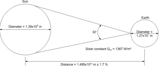
The data is then used to model the performance of the parabolic trough, compact linear Fresnel reflector, center receiver and dish motor technologies. Carnot efficiency - Dish motor receiver with equivalent radiation conduction W/mK Extraterrestrial radiation striking a plane perpendicular to the.
INTRODUCTION
- Project summary
- Motivation for project
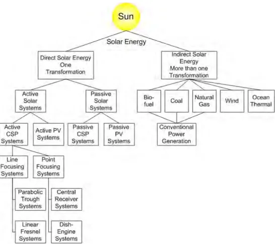
- Solar energy technologies
- Concentrating solar power technologies
- Parabolic trough systems
- Linear Fresnel systems
- Central receiver systems
- Dish-engine systems
- Solar energy technology assessment methods
- Structure of dissertation
South Africa has one of the highest levels of carbon dioxide emissions per capita in the world.” It defines direct solar energy as usable energy harnessed after just one transformation of sunlight in its natural form.
LITERATURE REVIEW
Introduction
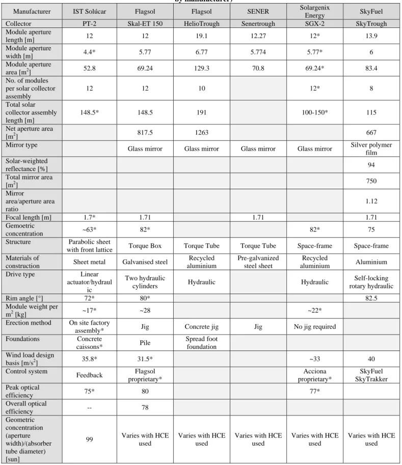
Parabolic trough systems
- Reflective parabolic collectors
- Linear tubular receivers
- Heat transfer fluids
- Thermal energy storage
- Power plants
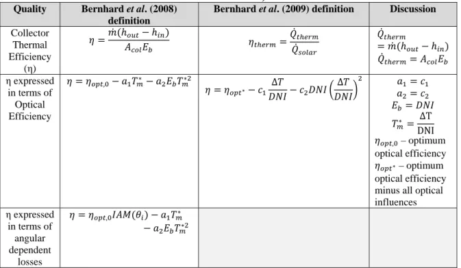
One factor that acutely affects the efficiency of a linear tubular receiver is the stability of the vacuum in the annulus. One of the central design considerations in Rankine cycle CSP applications is the heat removal system.
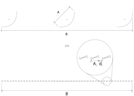
Linear Fresnel systems
- CLFR optic and thermal efficiencies
- Absorber configuration
- CLFR power plant
The first is a vertical linear tubular receiver mounted in the center of the primary reflectors. Due to the height of the absorber, heat can be lost if the wind blows past the absorber.
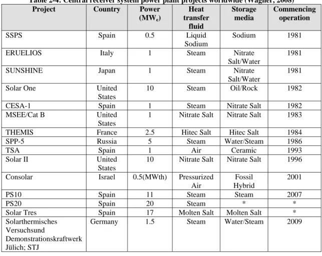
Central receiver systems
- Molten salt technology
- Open or closed loop volumetric air technologies
- Saturated steam technology
- The heliostat field
- The central receiver
- Power cycle technology
A useful summary of CRS molten salt power plant operating modes is provided by Burgaleta et al. The placement of the heliostatic array is an integral part of the CRS design.
Dish-engine systems
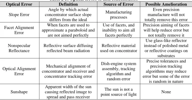
- Concentrating dish collector
- Solar receiver
- Engines
- Overall system
It is the current intensity at a point on the receiver divided by the insolation on the concentrator as reported by Stine and Diver (1994). When the receiver output power supplied to the Stirling engine ( , ) is given by the previously defined solar power intercepted by the receiver ( , ) minus the amount of radiation reflected from the receiver aperture ( , ), the receiver conductance loss .
SOLAR ENERGY AVAILABILITY AT UPINGTON
Introduction
Here, the accuracy, spectral sensitivity and regular calibration of the pyranometer determine the correctness of the resulting global and diffuse irradiance data. Bekker (2007) proposes the following classification system (Table 3-2) for grading the accuracy and resolution of solar radiation data.
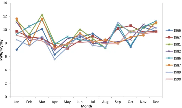
Data analysis
- SAWS pyranometer data
- NREL CSR model data for Africa
- NASA SSE global dataset
- Eskom Sustainability and Innovation Department data
- Weather Analytics data
- CRSES data
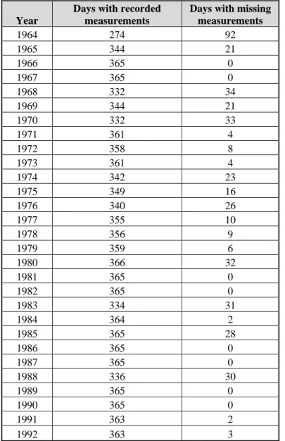
If no ground-based measuring station exists, satellite measurements are the only indication of the amount of solar energy at a location in question. However, upon inspection, it was found that numerous days contained missing data and in some cases identical measurements were recorded for several consecutive one-hour periods, casting doubt on the overall quality of the data set. Although it is not possible to verify the accuracy of the measurements, the uncertainty associated with the data is unlikely to fall within the expected 2%.
A point of interest is that one of the BSRN gauging stations used to determine the accuracy of the SSE data set was at De Aar, which is approximately 350 km from Upington and has very similar meteorological conditions. The work involved in setting up and operating the station is detailed by Esterhuyse (2004). A detailed description of the methodology used to arrive at the dataset is provided by NASA (2009).
Some stations have long gaps in their data logs (many missing data points) due to "equipment failure" (Eskom, 2010b, 1), which is believed to be due to tracker and power supply problems. A typical meteorological year for Upington produced by METEONORM in EPW format was made available to participants in the CRSES Solar Advisor Model CSP and PV simulation software training from 1 June 2011 to 2 June 2011.
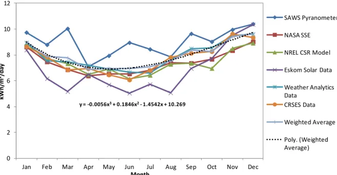
Calculation methodology and results
- SAWS pyranometer calculations
- NREL CSR model calculations
- NASA SSE calculations
- Eskom data calculations
- Weather Analytics data calculations
- CRSES data calculations
- Results
- Modelling considerations
The second part of the calculation was to relate each hourly measurement of total and diffuse radiation to the basic geometric relationships described in Appendix A, including declination, solar time, hour angle, zenith angle, and sunset hour angle. The difference between the two results was largest at the beginning and end of the year and smallest in the middle of the year, towards August. The distribution of the difference was reminiscent of a normal distribution with the fewest errors normalized around the middle of the year and the largest errors found at both extremes of each calendar year.
The output of the model for the 40 by 40 km cell including Upington is shown in Figure 3-3 below. These findings were problematic because the average radiation presented here is determined cumulatively, so replacing missing data points with zero values to get a more accurate representation of the "as is" data results in a suppressed average. Using an average of the six predicted DNR levels, the South African solar resource compares extremely well with several international CSP locations (Table 3-5).
This result agrees well with the estimate of the location of the solar source at the Upington Solar Park by Suri et al. 2011) from GeoModel Solar combined four years (November 2006 to February 2011) of ground-based measurements from Eskom and Stellenbosch Universities with seventeen years (1994 to 2010) of solar radiation data obtained from the SolarGIS satellite to estimate DNR, GHI and global tilt irradiation. at an optimal angle of 28°. SAM requests hourly data for one or a typical year of measurements listed in Table 3-8.
MODELLING AND RESULTS
Introduction
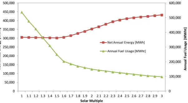
Intra-technology simulation results
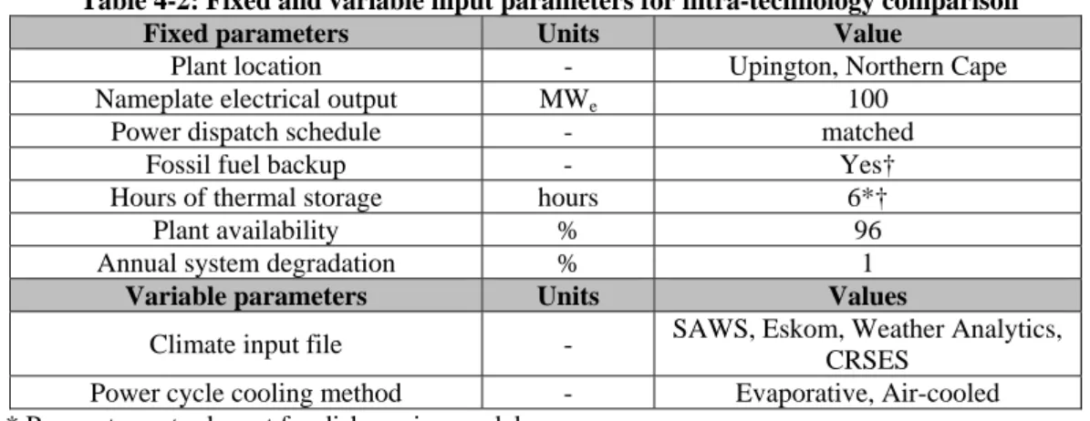
- Global model parameters
- Parabolic trough simulation
- Parabolic trough simulation results
- Central receiver simulation
- Central receiver simulation results
- Dish-engine simulation
- Dish-engine simulation results
- CLFR simulation
- CLFR simulation results
The power cycle transmission settings of the linear Fresnel model were matched to the parabolic trough and power tower settings. The cooling system used for the power block determines the annual water consumption of the installation. SAM provides a wizard for circular field optimization in the heliostat field component model of the power tower model.
As mentioned in section 4.2.2.4, the power cycle component model for the physical trough model is the same as that used in the power tower model. The gross to net conversion factor of the central receiver system is less affected by the power cycle cooling method than the parabolic trough system. As previously mentioned, the ground requirement for the central receiver is significantly higher than the parabolic trough.
Given Upington's average annual wind speed of approximately 3.6 m/s, the plant is not expected to experience wind speed related disruptions. A dispatch control component is included in the power cycle component of the linear Fresnel model, as it does not have a TES component model.
Inter-technology comparisons
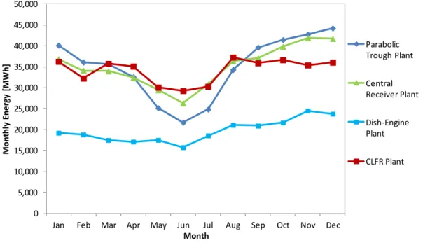
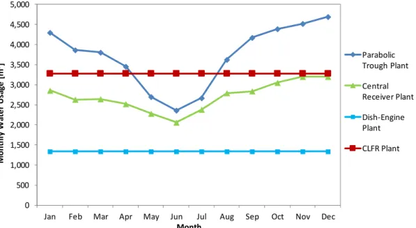
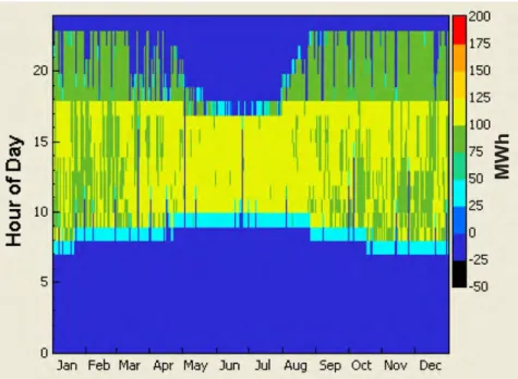
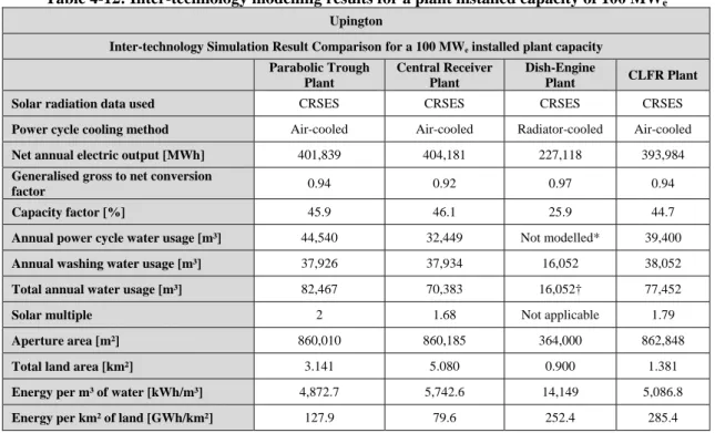
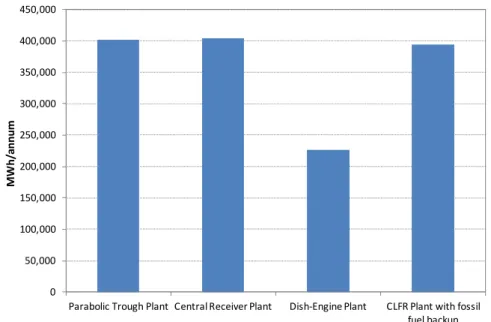
The results show that central receiver and parabolic trough technology provide more electrical energy than their CLFR and parabolic trough counterparts. However, the parabolic trough system used significantly more water annually than the central receiving system (17.2% higher annual water consumption). The results show that central receiver technology best meets the requirement for evening load peaks in the national load profile.
The CLFR plant does not match the national load profile as well as the central receiver or parabolic trough plant. Removal of fossil fuel backup illustrates how the higher optical efficiencies achievable by the parabolic trough and central receiver affect their net annual electrical output as opposed to the linear Fresnel model. The difference between the central receiver and the linear Fresnel net annual electrical production grows from 2.6% to 48.6% when fossil fuel backup is removed.
The difference between the parabolic trough and the central receiver's net annual electrical output increases from 0.6% to 1.1% when fossil fuel backup is removed. However, the uncertainty regarding Stirling Energy Systems – the manufacturers of the dish engines modeled in this study – as well as this system's lack of TES which limits its ability to track the national load profile, are both significant drawbacks to its implementation.
Validation of simulation results
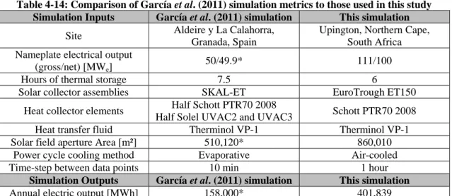
- Parabolic trough result validation
- Central receiver result validation
- Dish-engine result validation
- CLFR result validation
They found that the annual collector efficiency of the parabolic trough was 55.8%, while the CLFR yielded a value of 45.8%. The parasitic losses of the CLFR installation were lower than those of the parabolic trough installation. Therefore, especially at high solar incidence angles, the CLFR installation is unable to match the optical efficiency of the parabolic trough installation.
This resulted in reduced operating time for the plant, which in turn led to the lower annual electrical output of the CLFR plant compared to the dish-trough plant. With fossil fuel backup, the capacity factor for the parabolic trough plant is 2.7% higher than the CLFR plant. By removing the fossil fuel backup, the capacity factor of the CLFR plant becomes 32.6% lower than the parabolic trough plant.
Nevertheless, its final annual net electricity generation is still lower than the central receiver and parabolic dish models. Removing the reserve fossil fuel results in the CLFR plant model producing 32.6% less net annual electricity generation than the parabolic trough plant model.
DISCUSSION OF RESULTS
Solar resource assessment result
Modelling results
While the central receiver results differ from Wagner's (2012), the design parameters easily account for these differences. Therefore, the result of the central receiver model can be considered within the range of the SAM simulation results obtained by Wagner (2012) and Turchi et al. This reduces some of the advantages of the parabolic trough and the higher optical efficiency of the central receiver.
The removal of reserve fossil fuel from all three models caused the net annual production of the CLFR model to become significantly lower than that of the parabolic trough and central receiver. Parabolic trough plant Central receiver plant CLFR rotary engine plant Backup fossil fuel plant. The CLFR model produces 2% less electricity per year than a parabolic trough installation and 2.6% less than a central receiver when all have fossil fuel backup.
The overall efficiency of the CLFR is 32% lower than the parabolic trough and 33% lower than the central receiver model (Figure 5-3). The dishwasher model produced 44% less electricity annually than the central receiver model (Figure 5-1), but it also used 77% less water excluding radiator coolant water (Figure 5-4).
CONCLUSION AND RECOMMENDATIONS
Eight cases of the parabolic trough plant were modeled to evaluate evaporative and air-cooled plants based on the four DNI datasets. Gamble and Schopf (2009, p. 1) of Solutia Inc claim that Therminol VP-1 is “the most thermally stable organic heat transfer fluid available”. Dirt on the solar field mirrors significantly reduces the energy absorbed from the solar field.
In the plant capacity section of the power cycle interface SAM subtracts 10% from the gross electrical output to account for parasitic losses. The main inputs used in each component model of the power tower model are listed in the following sections. The solar manifold was positioned to provide an aperture area as close as possible to that of the modeled parabolic trough plant.
The evaporative and air-cooled settings were identical to the parabolic trough box. The parasitic loads for the central receiver were similar to that of the parabolic trough except for the following items. System Advisor Model calculates plant capacity by summing the nameplate capacity of each dish motor system in the solar array.
The parasitic loads for the CLFR plant were similar to that of the parabolic trough except for the following item.
![Figure 3-1: Average annual and monthly solar energy received per horizontal square metre [MJ/m2] (SARERD, 2006)](https://thumb-ap.123doks.com/thumbv2/pubpdfnet/10638337.0/66.892.163.731.339.728/figure-average-annual-monthly-energy-received-horizontal-sarerd.webp)