Details of contributions to publications included in the research presented in this thesis. Their work provides insight into the thermodynamic behavior of the stellar fluid and the effect of shear on the relaxation time during the collapse process.
Introduction
In this chapter we follow a treatment similar to that of Govender [52], except that our energy-moment tensor is load-free and is extended to include shear viscosity and bulk viscosity.
Vectors, covectors and tensors
Vectors
Covectors
It can easily be shown that applying ˜P to a vector V⃗ will give the scalar output it gives.
Tensors
Geometry of curved spacetime
When we contract the Riemann tensor (2.3.3), using the metric tensor gap, we get the Ricci tensorRab given by. The Einstein curvature, a rank two symmetric tensor, obtained from the Ricci tensor and the Ricci scalar, is given by
General overview of the energy momentum tensor
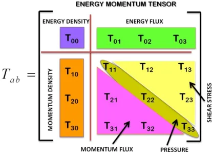
Rabcd = Γabd,c−Γabc,d+ ΓaecΓebd−ΓaedΓebc. 2.3.3) When we contract the Riemann tensor (2.3.3) using the metric tensor gab, we get the Ricci tensorRab given by Tab represents the ath component of the force per unit area (shear stress) over a surface with a normal in the bth direction (a̸=b).
Spherically symmetric spacetimes
- Line element
- Christoffel symbols
- Ricci tensor components and Ricci scalar
- Einstein tensor components
- Energy momentum tensor: Imperfect fluid
- Kinematical quantities
It should be noted that the energy density ρ comprises the rest energy of the mass. It can be easily shown that the nonzero components of the shear tensor are σ11 = 2.
Einstein’s field equations: Shearing spacetimes
The nonzero components of the Bianchi identities, Tab;b = 0, yield (in the absence of bulk viscosity and shear viscosity).
Field equations: Shear-free spacetimes
For pressure isotropy, we set ∆ = 0 in equation (2.7.3), which effectively equates the radial and tangential pressure. This condition must be solved to describe the internal matter distribution and the physical behavior of the system.
Exterior spacetime: Vaidya atmosphere
The solutions to Einstein's field equations for both inner and outer spacetime can be "glued" together to produce a complete picture of the collapse process. The criteria for smooth matching or continuity of the interior and exterior solutions are due to Darmois [60], Lichnerowicz [61] and O'Brien and Synge [62].
Shearing spacetimes
- Matching: Interior spacetime Z − to the hypersurface Σ
- Matching: Exterior spacetime Z + to the hypersurface Σ
- Summary: The first junction condition
- The second junction condition: Matching curvature
- Summary: The second junction condition
- Junction conditions: Shear–free limit
- Physical interpretation of equation (3.1.24b)
- Luminosity and surface redshift
This involves a smooth matching of the coordinates that describe the inner space-time to the coordinates on the (time-like) hypersurface, which is then matched to the outer space-time. Therefore, there are necessary and sufficient conditions for space-times to fulfill the second junction (3.1.2).
Perturbations for shearing spacetimes
In all these studies, the static model was assumed to be the isotropic Schwarzschild interior solution. These equations generalize the recent work of Herrera et al [78] in which they considered a similar perturbative scheme with vanishing heat flow for the expansion-free state. Surprisingly, they found that in expansion-free collapse “the range of instability is determined by the local anisotropy of pressure and the energy density.
The temporal equation employed in the perturbation scheme
Dynamical instabilities
Non-adiabatic spherical collapse
Herrera et al [18] studied the effect of heat flow on the dynamic instability of a shear-free fluid distribution with isotropic pressure and no zero radiation. Analyzing (4.4.2), it becomes clear that the unstable interval of Γ increases with the Newtonian term (first term within the square brackets) as well as with the relativistic corrections (second term within the square brackets) that arise from the static fluid configuration. However, relativistic corrections due to heat flow (dissipation) (last term in square brackets) lower the unstable region of Γ.
Radiating anisotropic collapse
It is quite clear from (4.4.3) that the contribution of anisotropy to the unstable region Γ depends entirely on the sign of the difference between the static radial pressure pro. A difference (pto-pro) < 0 will reduce the instability of the system, while a difference (pto-pro) > 0 will increase the instability. Relativistic corrections (the second term in square brackets) increase the unstable region of the adiabatic index, resulting in unstable configurations.
Shearing viscous collapse
The rest of the contributions are all negative, resulting in a decrease in the instability of the system. Our use of the Cattaneo [27] equation or the Maxwell–Cattaneo equation, a truncated version of the Israel and Stewart [84] theory, is motivated in detail by Joseph and Preziosi [85] . Conservation of energy and momentum is achieved by setting the divergence of the energy-momentum tensor equal to zero, i.e.
Overview of irreversible thermodynamics for dissipative relativistic fluids 53
The equation describing the time evolution of entropy is obtained using the Gibbs equation (5.2.8), the number conservation equation (5.1.3) and the energy conservation equation. Eckart's theory of irreversible thermodynamics is appropriate in the Newtonian regime. However, the theory suffers from a violation of causality, which becomes apparent when we suddenly "turn off" the thermodynamic force on the right-hand side of equation (5.3.8), causing the heat flow to instantly disappear. It is easy to see that after setting the relaxation time coefficient τ1 to zero in (5.4.9), we obtain the Eckart heat transfer equation (5.3.8).
Thermodynamics in relativistic stellar fluids
- General case
- Non–causal solutions: ψ = 0
- Causal case: ω = 0
- Causal case: ω = 4
An abbreviated form of the Israel–Stewart causal heat transfer equation (5.4.5) is the Maxwell–Cattane equation (5.4.9), which is expressed as They were able to show that the inclusion of the total viscosity reduces the effective adiabatic index within the stellar core, thereby increasing the instability of the collapsing star. The purpose of this chapter is to highlight the effect of shear on the temperature profiles of the decaying matter distribution.
Interior spacetime
Exterior spacetime and junction conditions
The continuity of the intrinsic and extrinsic curvature components of the inner and outer space times across a time-like boundary yielded equations (3.1.24a) and (3.1.24b). In the absence of bulk viscosity, free steam radiation and shear viscosity, the junction condition (3.1.24a) remains the same, i.e.
Temporal evolution
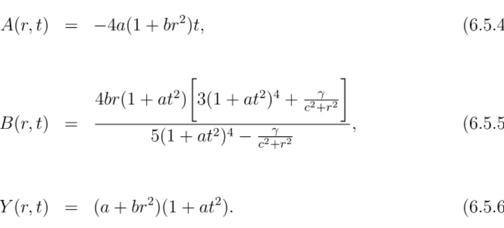
With an insightful choice of f(r), we can investigate the role that shear force plays directly on the collapse process. It is striking that we can write down the kinematic and thermodynamic quantities in compact, closed form.
A particular radiating model
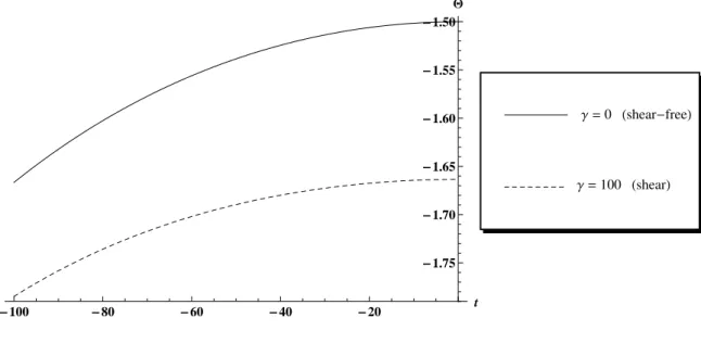
We have been able to achieve this because our model allows us to switch off the shear and compare the physics in both the shear and shear-free limits. The opposite trend is observed at the center of the collapsing star, that is, the collapse rate in the presence of shear is lower than the collapse rate in the case of shear, as shown in Figure. It is worth noting that the effect of shear The collapse rate at the boundary is of the order of 103 times smaller than at the center.
Causal thermodynamics
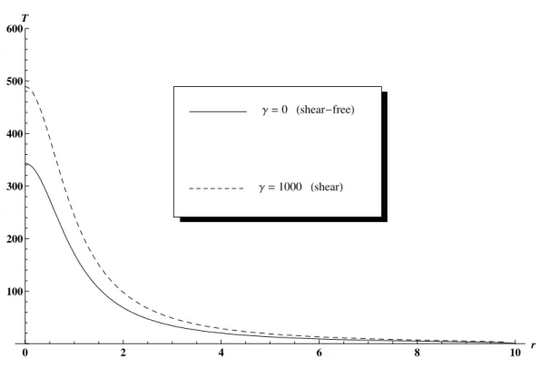
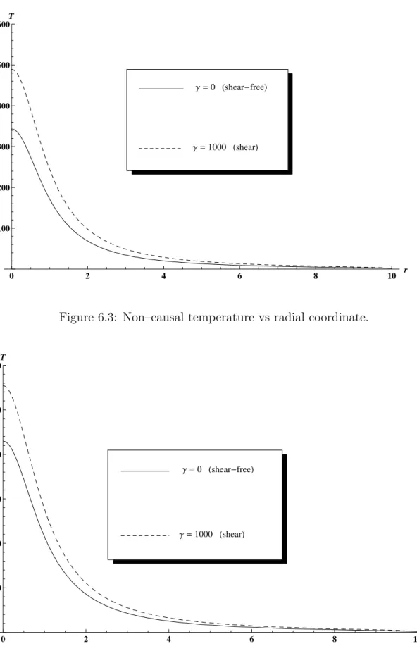
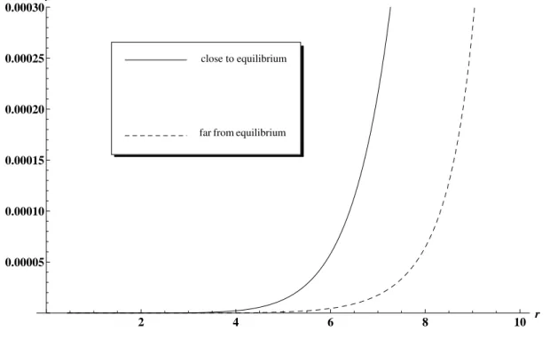
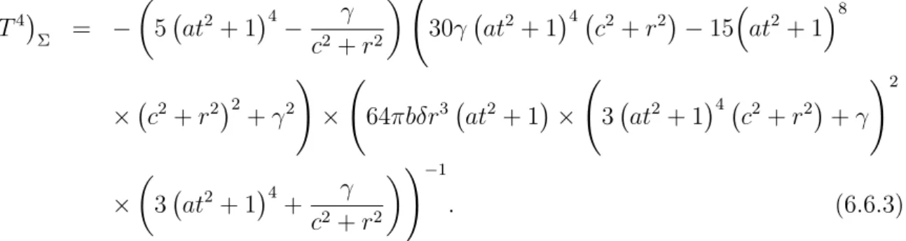
We can understand the increased temperature in the core of the star from the fact that the displacement is responsible for the internal friction between the layers of the stellar fluid. This interaction between the layers at each interior point of the colliding body leads to the generation of heat within the core. The trend in the brightness profile in relation to the displacement can be understood from the deviations from the displacement-free profile.
Proper radius
With appropriate choices for a, b, c, and γ in (6.7.1), we find that the appropriate radius Rp decreases with time, which is reasonable because the star collapses gravitationally and loses mass and energy. For high values of γ we see that after a certain time the radius of the star begins to increase, implying that the star begins to expand. One possible explanation is that the high degree of shear (due to γ) causes such intense internal friction that the stellar fluid heats up significantly, resulting in enormous heat flux and hydrodynamic pressure that can significantly overcome gravity.

Stability analysis of the model
In other words, the presence of shear during the final stages of collapse makes the fluid 'softer' and therefore less susceptible to gravitational collapse. At the boundary, the shear contributes positively to the hydrodynamic forces that compete with gravity to keep the stellar fluid stable. The remaining terms in (4.4.6) are negative and have a collective effect larger than the single positive term, implying that the inclusion of shear is successful in stabilizing the star fluid distribution against collapse.

Conclusion
In §7.2 we present the field equations that describe the geometry and matter content of a star undergoing gravitational collapse. In §7.3 we discuss the perturbative scheme as well as the static and perturbed quantities, including the expansion coefficient, shear force and mass functions. In §7.4 we present the conditions for a smooth coordination of the internal spacetime with Vaidya's external solution across a time-like boundary.
Shearing spacetimes
Perturbative scheme
Exterior spacetime and junction conditions
The temporal equation employed in the perturbation scheme
When these factors are taken into account, the temporal evolution equation for our model is then given by
The static core
We simply state the equations here and discuss the relationship between the anisotropy parameter ∆ and the anisotropic factor C. It is also worth noting that the ratio of the anisotropic critical mass to that of the isotropic case is given by. Furthermore, the radial pressure at any interior point of the star distribution increases as the relative anisotropy increases (larger h values).

The nonstatic model
It is also clear that the degree of anisotropy increases the perturbations of the radial pressure, and this effect is more pronounced near the center of the stellar fluid. Again, we note that the perturbations in the tangential pressure grow with increasing deviation (larger h) from isotropy (h = 1). 7.11–7.12, where it is clear that the perturbations to the displacement close to the core are enhanced as the anisotropy increases.

Stability analysis
This indicates that the core region of the star is less stable than the cooler boundary layers. This is due to the fact that a transformation of the Bowers and Liang metric from curvature coordinates to moving isotropic coordinates is required. It will also be valuable to study the effect of the anisotropic factor on the relativistic contributions to the stability or adiabatic index.
Thermal behaviour
To this end, Govender et al [39] have investigated the causal and non-causal profiles of the perturbed temperature in the linear perturbation regime. Their results show that the perturbed temperature is higher in the causal case, implying that relaxation effects increase the temperature contributions due to perturbations. Recently Govender et al [40] have demonstrated that logging increases both causal and non-causal temperature profiles, and that causal profiles are higher than the non-causal case in both logging and non-logging cases .
Perturbation of the temperature
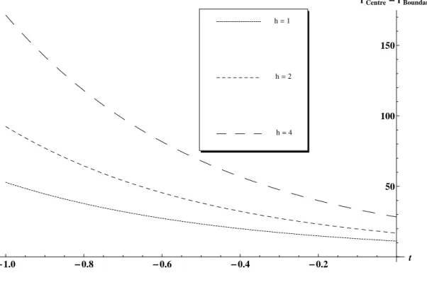
Using the parameters of our static model in (7.10.2), we obtain an expression for the perturbed temperature in terms of the anisotropic scale factor h given by . Herrera and Santos [83] and Maharaj et al [39] provide a discussion of the physical meaning of equation (7.10.4), which was first obtained by Tolman in 1930. The perturbed temperature profiles for different degrees of ether anisotropic parameters are shown in fig.

Conclusion
Our results in Chapter 6 clearly illustrate that the inclusion of shear results in higher temperature, which is more pronounced in the core regions of the star as opposed to the surface layers. We believe that gravitational collapse still holds many secrets that we have yet to uncover. 109] W Baretto, L Herrera and N Santos, A generalization of the concept of adiabatic index for non-adiabatic systems, Astrophys.