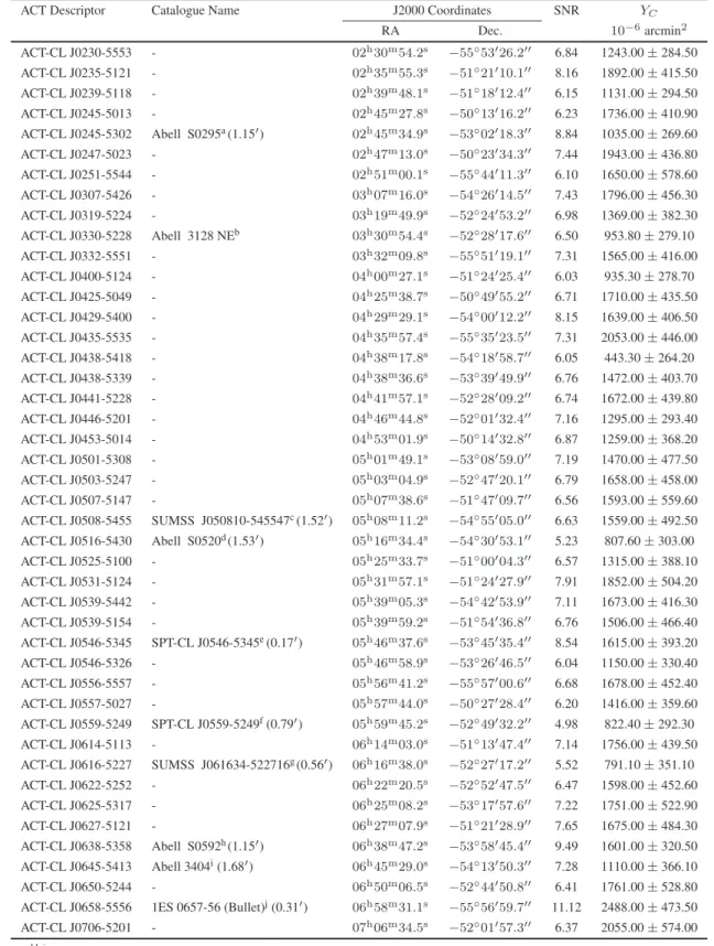
The fifth chapter in this thesis deals with the first results of the Atacama Cosmological Telescope Project. The first detection of the SZE using an interferometer was made with the Ryle Telescope (RT), located in Cambridge, England (Jones et al., 1993).
The Standard Model of Cosmology
The motion coordinates are related to the appropriate length measure,x, byx(t) = a(t)r, where (t) is the scale factor of the universe. This event defines a surface in the thermal history of the universe, which is often called the "surface of last scattering", since at this point the electron-photon interaction length exceeded the scale of the universe.
Large Scale Structure Formation and Growth of Clusters
- Density Perturbations
- Growth of Linear Perturbations
- The Cold Dark Matter Power Spectrum
- Spherical Collapse
- Cluster Mass Profiles
- Cluster Mass
- Cluster Mass Function
To understand how density perturbations give rise to large-scale structure formation, we need to understand the physical meaning of the perturbation spectrum P(k). Furthermore, if the dark energy is negligible, the radial behavior of the shell is determined by the following parametric equation.
Cluster Probes
Clusters in Optical Light
Optical observations provide the opportunity to cover wide areas of the sky with large CCD frames coupled to telescopes with large fields of view. In addition, studies of the colour-magnitude ratio in red galaxies have enabled accurate distance measurements of clusters out to ~1 (Gladders and Yee, 2005).
Clusters in X-rays
Furthermore, if one makes the assumption that the universe is of the Einstein-de-Sitter form, then ∆v is constant, and the temperature of an isothermal gas distribution is related to the mass byT ∝M2/3(1+ z). Today we are in the era of XMM-Newton and Chandra satellites, which together with the large survey area of XMM-Newton and the high angular resolution of Chandra have begun to shed light on the interplay between the complex dynamics of the intra-cluster medium and the detailed physics of star formation.
Clusters in the Microwave
Since the first attempts in the 1970s to map the X-ray sky (Giacconi et al., 1979), observations in this wavelength band have been prolific. Numerous studies in the 1990s, such as those using the ROSAT satellite, have helped to constrain cosmological parameters (see Rosati et al., 2002, for a review of several cosmologically significant X-ray studies).
The Sunyaev-Zel’dovich Effect
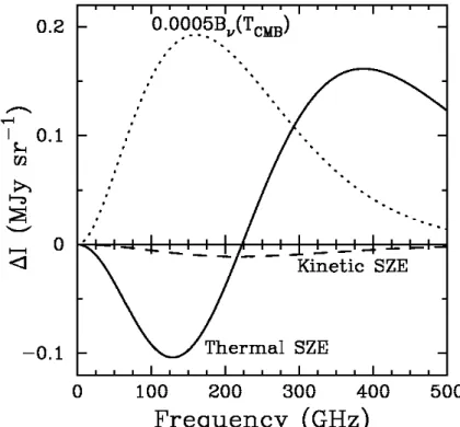
Thermal Sunyaev-Zel’dovich Effect
The Compton parameter yc in Eq. 2.4.40) is the measure of the gas pressure integrated along the line of sight. The derivative of the blackbody with respect to temperature,|dBν/dT|is the coupling factor between TtSZ and∆ItSZ.
Kinetic Sunyaev-Zel’dovich
The gas pressure inside clusters is an excellent measure of the gravitational potential, and YSZDA2 is therefore expected to be closely related to the cluster mass. The salient features of the tSZ are: (1) it is a weak distortion of the CMB spectrum that is proportional to the cluster gas pressure along the line of sight; (2) the effect is independent of redshift; (3) it consists of a unique frequency dependence (with a decrease of the CMB intensity for frequencies < 218 GHz, null effect at the null ≈ 218 GHz, and an increase of intensity for frequencies higher than the zero); (4) the total tSZ signal is proportional to the inverse of the squared angular diameter distance, implying that SZE surveys will contain redshift-independent thresholds, especially at high redshifts.
Observations of SZE Clusters
The Atacama Cosmology Telescope
These include tackling the shortage of baryons in the local universe, and trying to understand the dynamics of clusters and their formation. In this thesis we investigate the performance of ACT and other next-generation experiments, and impose constraints on cosmological parameters through the analysis of clusters and groups of galaxies.
South Pole Telescope
PLANCK
This catalog will be invaluable in studies of cosmological models and our understanding of the evolution of large-scale structure. In the following chapters we present studies of galaxy clusters thus providing an insight into their properties and applications in cosmology.
Introduction
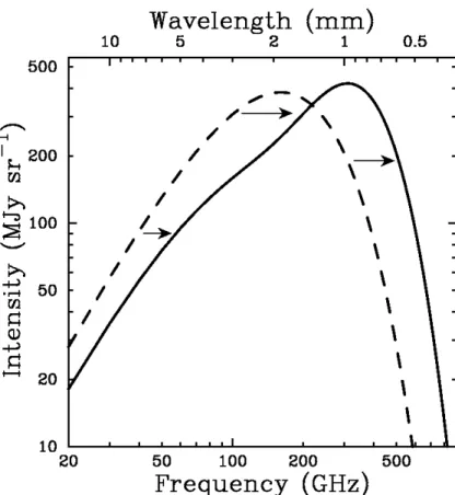
The population of hot electrons in the cluster gas energizes photons in the Rayleigh-Jeans part of the spectrum which push them into the Wien tail. However, a new generation of high-resolution CMB experiments with superior detector sensitivity offers the hope of detecting and constraining the properties of the hot gas in galaxy clusters.
Hot Gas Halo Models
Dark Matter Halo
The exact dependence of the concentration parameter on mass and redshift is still uncertain as several parametrizations have been used in the literature (e.g. As previously observed (Komatsu and Seljak, 2002) we find, however, that our results are insensitive to the exact choice of the concentration parameter .
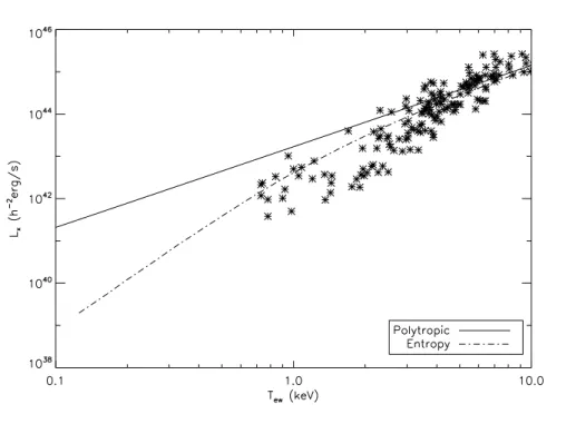
Polytropic Model
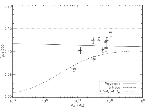
The temperature at the virial radius is close to the virial temperature and the central and average temperature has been found slightly higher (e.g. Frenk et al. Furthermore, there is good evidence that fgas(< . r200) converges to the universal baryon fractionfb(Vikhlinin) et al., 2006; Sanderson et al., 2003;.
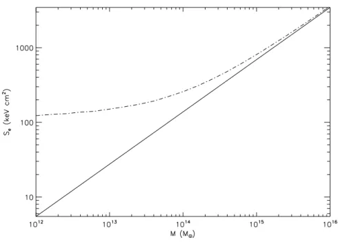
Entropy Model
We normalize the gas density by assuming that the gas pressure at the virial radius remains unchanged due to the entropy injection, which means we assume that the gas returns to pressure-balanced hydrostatic equilibrium at the virial radius after the energy injection.
Multi-Frequency Filtering of the Halo tSZ Signal
- Multi-Frequency Wiener Filter
- Halo Thermal Sunyaev-Zel’dovich Signal
- Foreground Components
- Detector Noise and Experimental Specifications
The top right panel shows the power spectra of the residual tSZ background and the residual Galactic dust. The lensed CMB angular power spectrum is shown in Figure 1CAMB: http://www.camb.info. 3.3 Multi-frequency filtering of the Halo tSZ 66 signal.
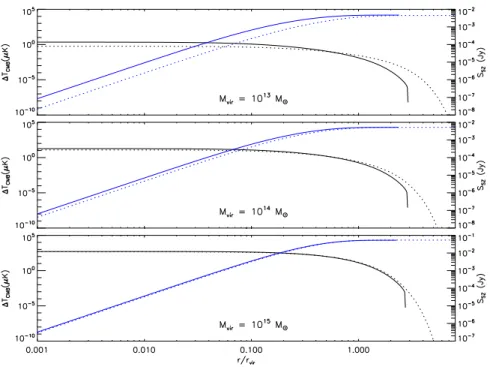
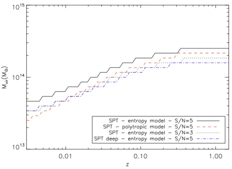
Detectability of the Halo tSZ Signal
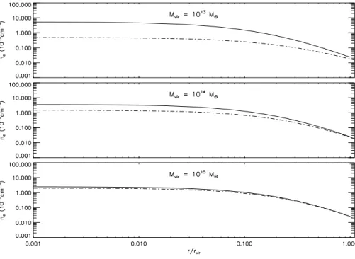
The minimum detectable mass is plotted for the entropic model with S/N = 5 (solid curve) and S/N = 3 (dotted curve) and the polytropic model with S/N = 5 (dashed curve) for the nominal SPT survey. The minimum detectable mass is plotted for the entropy model with S/N = 5 (solid curve) and S/N = 3 (dotted curve) and the polytropic model with S/N = 5 (dashed curve).
Discussion and Conclusions
Here again, a large-volume cosmological simulation will help quantify the impact of the tSZ background on the detection of group haloes and their recovered flux. In combination with existing optical and X-ray observations of these haloes, these measurements will increase our knowledge of the physics of galaxy formation and its effect on the intragroup medium.
Introduction
In light of this, Pace et al. 2008) presented analyzes of SZ and X-ray cluster detections using single- and multi-band filtering applied to simulations involving gas dynamics as well as other processes including feedback, star formation and radiative cooling. Another source of scatter in the SZ flux–mass scaling relation is flux measurement error caused by projection effects ( White, 2001 ; Holder et al., 2007 ; Hallman et al., 2007b ).
The Sunyaev-Zel’dovich Effect
ACT Sky Simulations
The Microwave Deblender
The Map Deblending Algorithm
Second, the child templates are constructed by comparing the intensities of pairs of pixels located symmetrically around the peak pixel and replacing both by the lower of the two. The latter stage does not mean that the final mixed child contains any specific symmetry as shape symmetry is only enforced in the construction of the templates.
Statistics of tSZ Detections
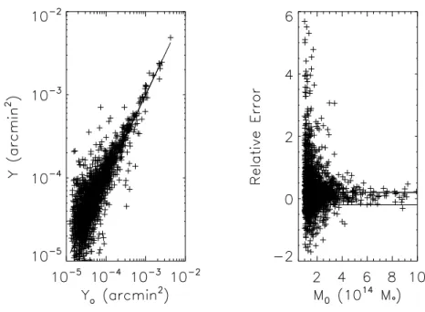
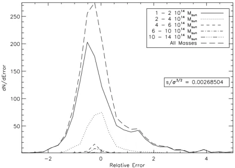
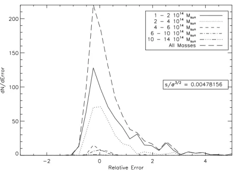
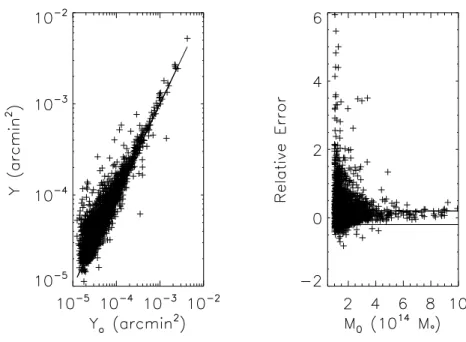
The skewness (presented as a dimensionless quantity rescaled to the standard deviation) of the total error distribution is also presented. In the bottom panel we express this error as a fraction of the mean SZ profile within the bin.
Physical Properties of Clusters and Groups
Statistics of tSZ Detections
The Wiener filtered 200 degree tSZ map for the ACT-Deep study is shown in the right panel of figure. In the next section we describe how the Compton profiles for each of the detected tSZ haloes were extracted from the maps.
Compton Profiles of tSZ Halos
As shown in §4.4, the unmixing process produces a more accurate radial Compton profile, especially in the outer regions of the cluster. This indicates that any biasing effect of the Wiener filter on the Compton profile is small.
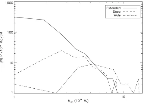
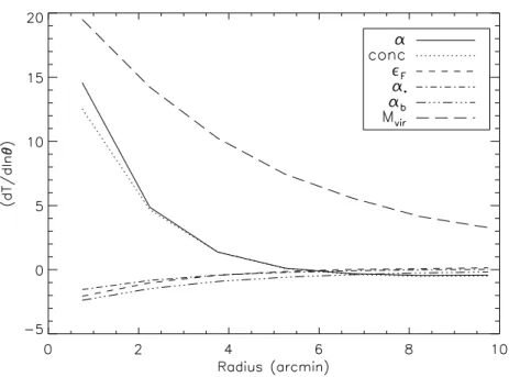
Constraints on Cluster Parameters
We note that the degeneracies between the cluster parameters in the case of the extended survey are somewhat orthogonal to the degeneracies between these parameters in the deep and wide surveys. The measurement of the stellar fraction and baryon fraction indices in the extended survey means that these observations will be able to measure a deviation from a constant scaling relation.
Discussion and Conclusions
In the second part of this chapter, we used a multi-frequency Wiener filter to obtain a map of the tSZ signal. In the case of Fisher matrix analysis, no parameters were previously estimated.
Introduction
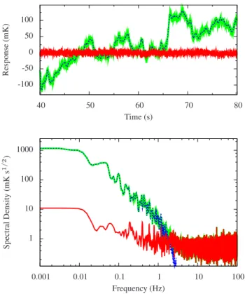
Although most of the atmospheric power is below the frequency of our 0.0978 Hz scans, on typical nights the atmosphere dominates the detector noise up to about 2 Hz. One of the most useful applications has been the study of our instrumental beam with high signal-to-noise maps of the planets.
The Cottingham Mapping Method
- The Algorithm
- Discussion
- Spatial Structure in the Atmosphere
- The B-Spline as a Model of Atmospheric Signal
- Implementation
- Map-Making
Given a set of basis functionsB, the Cottingham method minimizes the variance of the map pixel residuals with respect to the amplitudes α. The small residual atmospheric–celestial covariance manifests as streaks along lines of constant height, since with our 7◦ peak-to-peak, 1.5◦s−1 azimuthal scans (or 4.47◦ at 0.958◦s−1 when they are projected onto the sky at our observation height of 50.3◦), the nodal distance (τk = 1.0 for beam.
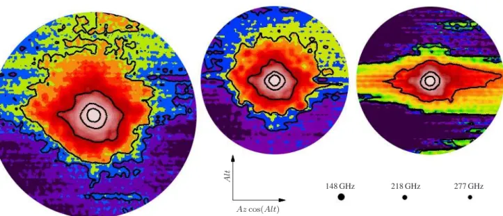
Beam Maps and Properties
Data Reduction
The mask sizes for the three arrays, whether used for band removal or background estimation, are listed in Table 5.1. The weights were determined from the RMS mean background level calculated outside the mask radius.
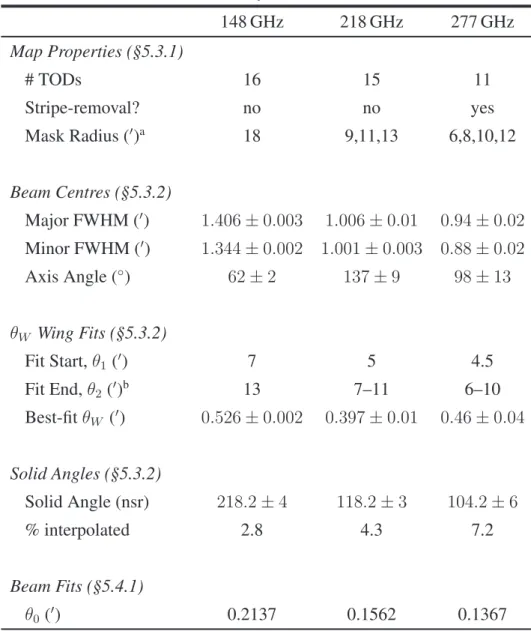
Beam Measurements
Determining the rest of the uncertainty in the solid angle is not straightforward, as systematic errors dominate. First, we calculated the mean and standard deviation of the solid angles measured in each map.
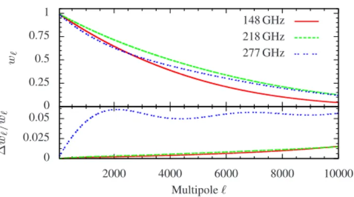
Window Functions
Basis Functions
In the case of an azimuthal symmetric beam, we only need to consider the m = 0 radial polynomials, which can be expressed in terms of Legendre polynomials, Pn(x)as: Motivated by this, we assume. 5.4.24) if we set basis functions to fit the radial beam profile.4 Here we set a fitting parameter, θ0, to control the scale of the basis functions.
Fitting Basis Functions to the Beam Profile
As input to the fitting procedure, we must specify the scale parameter, θ0, and the polynomial order, nmax.
Window Functions and their Covariances
Another source of systematic errors in the window functions comes from the fact that the beams are not perfectly symmetrical. The symmetric beam window function generally underestimates the power in the beam (e.g. Fig. 23, Hinshaw et al., 2007).
SZ Galaxy Clusters
- Data
- Characterising the Detections
- Integrated Compton-Y Values
- Comparisons to Previous Measurements
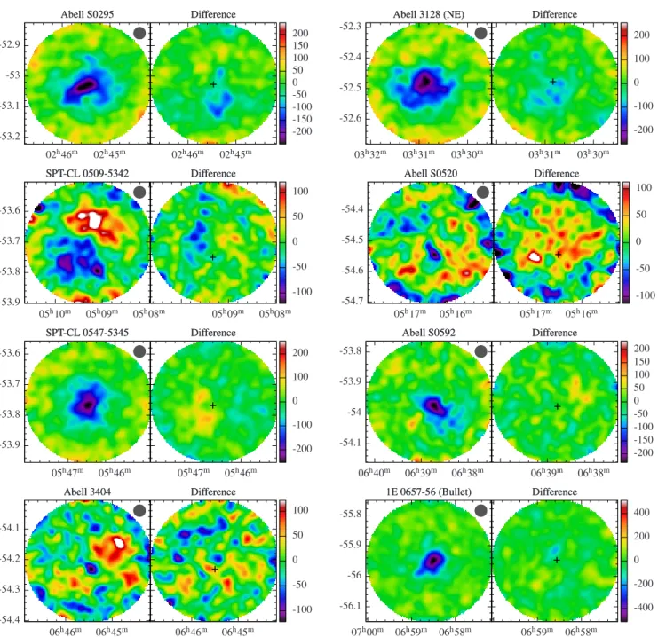
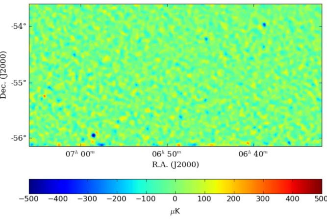
The rising and set difference maps are then coadded to produce the full cross-linked coadded difference map - the same procedure used for the signal maps. The units for the axes are right ascension (hours) and declination (degrees), and the color bar is ∆TCM B (µK).
Conclusions
Our high-σ detection of thez = 0.44 component of Abell 3128, and our current non-detection of the low-redshift part, confirm existing evidence that the further cluster is more massive. In this chapter, we present preliminary cluster detection analyzes of the latest ACT sky maps at 148GHz using the SZ effect.
Overview of ACT Data Maps
Overview of ACT Simulation Maps
Map Filtering
Instead of applying the Wiener filter in one dimension, as is usually the case assuming symmetry in the power spectrum of different sources, we have implemented a two-dimensional Wiener filter. To assess the impact of model selection on cluster detection, we also investigated the situation where the noise template included the power spectrum of the data instead of the theoretical models.
Detection Statistics: ACT and Simulated Maps
Considering the fact that we used the same source models (dust and lenticular CMB) in the construction of the simulated map, this behavior is not unexpected. Using the data in the filter construction produced a closer correlation between the actual and simulation number counts.
Flux Statistics: ACT and Simulated Maps
ACT Cluster Candidates
Conclusion
This information will be used to place constraints on normalization of the matter power spectrum,σ8, and matter density,Ωm. Furthermore, a measurement of the tSZ effect in the outskirts of such haloes would place constraints on entropy injection levels as well as the baryon fraction.
APPENDIX A
The panels from top to bottom show the entropy profiles for the halo masses Mvir and 1015M, respectively. The panels from top to bottom show the integrated brightness profiles for the halo masses Mvir and 1015M, respectively.
APPENDIX B
The dark matter velocity dispersion is defined as. 2.0.12), where σcis is proportional to the surface pressure. This model is similar to the one of the same name in Bode et al.
APPENDIX C
APPENDIX D
At the center of the beam, which is the apex, the gradient disappears. where µΨ2 is the second raw moment of the shape of the planet Ψ. In the small planet approximation we are making, the second term in the parenthesis is small.