Details of the detection method for turning points in the bull and bear markets are provided in Chapter 3, while data sources and collection methods are described in Chapter 4. Designing an algorithm to replicate turning points in the stock market is problematic because there is a lack of consensus on some of the turning points in the bull and bear markets. Pagan and Sossounov (2002) therefore adapted Bry and Boschan's (BB) algorithm for use in stock markets by consulting some of the earliest literature on bull and bear markets.
First, the data are not smoothed at all, since the large movements possible in stock markets are some of the most interesting data points, and smoothing the data may remove their effects (see also Canova 1994 and 1999).2 The window for identifying local peaks and troughs are extended to eight months on each side, and a cycle must last at least 16 months, while a phase is only required to last at least four months. Once the turning points have been identified, the characteristics of bull and bear markets are examined. An alternative and more complex method of identifying turning points in bull and bear markets is regime change.
Their analysis focuses on volatility shifts rather than dating bull and bear market turning points. Stock market studies that consider market trends but do not formally examine bull and bear markets include the return momentum literature. It is assumed that the statistical process for Rt is subject to alternating upward and downward bull and bear market shifts (average return) regime shifts of potentially varying magnitudes and timing, the time and magnitude of which are unknown. 3 The drift parameter (average return) It is assumed that µk is fairly stable within each bull or bear market phase k, but shifts by an amount ?t+j whenever a bull or bear market occurs.
First, points higher or lower than those in five months on either side are identified.6 Alternation of turning points is then applied by selecting multiple highs or lows.
Data sources and collection method
The original Bry and Boschan (1971) algorithm is also applied to (unsmoothed) New York Stock Exchange trading volume data to identify time periods of increasing trading volume that can be used to determine whether bull markets detected by the BB method follow increasing stock market activity and investor interest. Periods between trading volume peaks and troughs are periods in which trading volume generally increases, which is often considered a bullish indicator of stock market sentiment (see, for example, Gitman and Joehnk, 1996). Identifying periods of increasing volume facilitates the characterization of bull markets detected by the BB method.
Between August and November 1914, the New York Stock Exchange was closed due to the First World War. For the purposes of constructing the stock index, the index levels for these four months remain the same as the closing value for the previous month (July). This study follows the standard practice of using nominal capital returns to identify bull and bear markets.
Schwert (1990) reports that the variation in dividend yields is small relative to the variation in stock prices, so the cyclical nature of bull and bear markets can be expressed using capital returns. The total volume of stocks traded monthly on the New York Stock Exchange (NYSE) is used to include a measure of investor interest. This information is available from the New York Stock Exchange in the form of daily trading volume, so it is summed over calendar months to give the NYSE monthly trading volume.
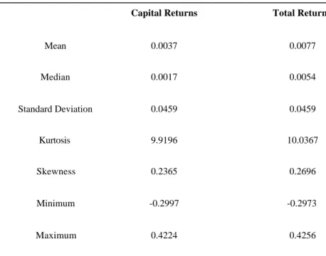
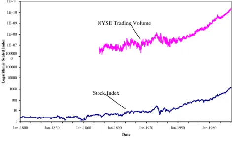
The level of the stock index and the NYSE trading volume series are shown in Figure 1. Both series show an overall upward trend over time, but large market movements such as the crash of 1929 are also evident. The average monthly capital return over the entire sample is 0.37% and the standard deviation of returns is 4.59%.
Empirical results
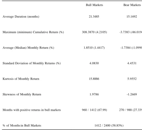
Two-thirds of months in bull states show positive stock returns, while less than a third of months in bear states have positive capital returns. A notable finding from Table 3 is that bull markets consistently exhibit a kurtosis of two to three times that of bear markets. This means that bull markets are more likely to see bigger moves, which means bull markets are likely to be more sensitive to outliers than bear markets.
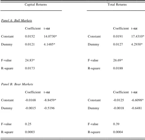
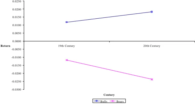
The results still show a doubling of the difference in average returns between bull and bear states from the 19th to the 20th century, so the effect is not just a result of the Great Depression (although the largest difference between bull and bear market returns occurs during the 1900 to 1950). For example, if only the first six months of a bull market phase have significantly high returns, then it may be that by the time a turning point is identified, the majority of the gains in a bull market have already occurred.11. They indicate that the first six months of bull markets show significantly higher returns than the remaining months of bull markets (e.g. 3.18% total return per results indicate that the remaining bull market months also produce very strong returns that are 1, 1% higher per month than the overall sample mean (see Table 1).13 In comparison, there is no significant difference in returns between the first six months and the remaining months of bear markets.
The results suggest that identifying turning points can potentially provide useful information for investors interested in market timing, especially since bull markets typically last much longer than six months (the average is 21 months). 1 1 It also takes six months to detect that a bull market is over, a consideration that would make it even more difficult to exploit turning points if most reversals in bull markets occurred during the first six months. 1 2 Note that the coefficient for the dummy represents the difference in average return between the first six months and the remaining months of a phase, and the constant represents the average return in the remaining months of the phase.
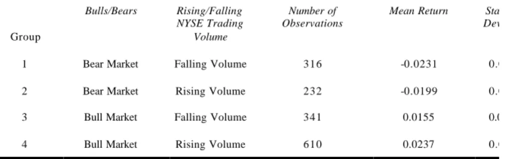
1 3 The latter finding closely approximates Maheu and McCurdy's explanation that the "majority" of bull market gains occur early in the phase, since a large proportion of bull markets tend to last at least two years. The interaction between bull markets and trading volume trend dummy variables is examined using two-way analysis of variance (ANOVA) of returns. Volume increases during bull markets and volume decreases during downtrends can be explained by investors' reluctance to sell losing stocks and relative haste to realize stock gains.
It can also be noted that while volume appears to provide little additional information on top of bull/bear classifications, the largest difference in mean returns is found between bull markets with increasing volume and bear markets with decreasing volume (see Panel B of Table 5). Casual observation of volume and index series shows that a volume peak often precedes the start of a bullish market (see Figure 1). More importantly, the result for the declining standard deviation of volume returns contrasts sharply with the small difference in overall volatility between bear and bull markets (see Table 3), thus suggesting that modeling approaches that identify markets of bears as high volatility conditions can focus on a bearish volume volatility. effect.
It may also explain why Maheu and McCurdy (2000) found that the stock market is in a bear market only 10% of the time, as bear market months with declining volume (and therefore much higher volatility) make up about 20% of the total. example in this study. The negative correlation between monthly volume trends and index volatility contrasts with the positive relationship between total volume and absolute index changes at daily time intervals (Ying, 1966), posing a challenge to theoretical explanations of the relationship between absolute price change of trading volume which has been developed to improve the everyday relationship (see for example Karpoff, 1987).
Conclusion
Canova, F., 1999, Does detrending matter for reference cycle determination and the selection of turning points?, The Economic Journal. Tong, 2000, The profitability of start-up strategies in international stock markets, Journal of Financial and Quantitative Analysis. Karpoff, J.M., 1987, The Relationship Between Price Changes and Trading Volume: A Survey, Journal of Financial and Quantitative Analysis.
McCurdy, 2000, Identifying bull and bear markets in stock returns, Journal of Business and Economic Statistics. Sossounov, 2002, A Simple Framework for Analyzing Bull and Bear Markets, Forthcoming in Journal of Applied Econometrics. Nelson, 1989, A Markov model of heteroskedasticity, risk and learning in the stock market, Journal of Financial Economics 25, 3-22.
The final phase is incomplete, so the average return for the phase is calculated using data through September 2000. Note that the cumulative return is the average of It,2/It , 1 –1, where It , 2 is the index level is at the level of the last stage. turning point that ends the phase and It,1 is the index level at the turning point that starts the phase. Dummy equals 1 if it is in the first 6 months of a phase, otherwise it is zero.
While the coefficient for the dummy represents the difference in average return between the first six months and the remaining months of a phase, the constant represents the average return in the remaining months of the phase.