1
Stock Exchange?
Martin P.H. Panggabean
Faculty of Economis Krida Wacana Christian University, Jakarta Email: mxpgyhoo@yahoo.com
ABSTRACT
Emerging participants in the Indonesia Stock Exchange (ISE) are the group of local retail players, characterized by small, frequent, and short-term trading activities that rely on market phases. Hence it is important for brokerage houses as well as the local retail players to enter the market at the appropriate moments. The goal of this paper, therefore, is to use regime-switching model using the weekly ISE index data to identify periods where the market is in a volatile period. Results from the calculation shows that the market is divided into two regimes: stable and volatile. Average length of period for each regime is 16 weeks and 10 weeks.
Keywords: Stock, regime-switching, maximum likelihood, retail investors.
INTRODUCTION
The Indonesia Stock Exchange (IDX, hence-forth) was formed in 2007 as a merger of two stock exchanges: The Jakarta Stock Exchange and the Surabaya Stock Exchange. The recent growth in the IDX activities has been quite rapid. In the past five years (2005-2009), trading volume, value, and frequency have increased substantially (Exchange, 2010).
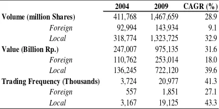
Table 1. Transaction Statistics in the Indonesia Stock Exchange, 2004-2009
2004 2009 CAGR (%)
Volume (million Shares) 411,768 1,467,659 28.9
Foreign 92,994 143,934 9.1
Local 318,774 1,323,725 32.9
Value (Billion Rp.) 247,007 975,135 31.6
Foreign 110,762 253,014 18.0
Local 136,245 722,120 39.6
Trading Frequency (Thousands) 3,724 20,977 41.3
Foreign 557 1,851 27.1
Local 3,167 19,125 43.3
Source: IDX (2010)
Table 1 shows the rapid growth of local players. Given that the number of shares increased by 32.9 percent while the trading frequency increases by 43.3 percent, we can conclude that more transactions are being conducted with smaller shares. This conclusion is in line with anecdotal evidences that saw more brokerage houses provide on-line trading system geared
toward these so-called retail investors. Even foreign brokerage houses are now offering on-line trading facilities to retail players. Thus the increase in the foreign transaction activities is to a certain extent caused by activities of retail players. These retail investors are known for their small and frequent purchases of stocks in the market. They are mostly short-term players that rely on market condition and phases to make their profits.
The basic intuition for market short-term trading is the belief that markets goes through phases. The term “Bulls and Bears” is an example of one such belief that the market has two phases. The market may have more than two phases. Nevertheless, each phase has its characteristics. Bears market, for example, is typically charac-terized as not only having negative rate of returns but also having high volatility as well. The opposite is true. Thus the connection between market phases and activity of short-term investors should be clear. Some short-term investor may get into the market (i.e. buy stocks) if the market is in the bullish period with positive expected rate of return. Other short-term investors may get into the market, even if the market is in the bearish phases, if they want to take advantage of the market volatility.
questions and thus provide guidance to short-term investors.
The origin of the regime-switching model itself dated back to 1973 with the seminal paper written by Goldfeld and Quandt (1973). However, given the non-linear nature of the model, popularity of the regime-switching method increases only recently through the existence of powerful computers.
The regime switching models has been applied in many fields. We will briefly survey several relevant articles in this field. A complete survey is beyond the scope of this paper. In the foreign exchange market, Norden (1995) uses regime-switching result as test for exchange rate bubbles using the Japanese Yen, German Mark, and Canadian Dollar. Norden and Vigfusson (1998) uses regime-switching model to detect exchange rate bubbles in the Japanese Yen, German Mark, and Canadian Dollar. Moerman (2001) used the regime-switching model to predict exchange rate rates of several major currencies such as US Dollar, UK Poundsterling, and Japanese yen. Alvarez-Plata and Schrooten (2003) uses the model to analyze the 2002 Argentinean currency crises.
In macroeconomics context, one example is the use of regime-switching model in analyzing New Zealand’s Gross Domestic Product (Buckle et al. 2002). Kumah (Kumah 2007) also uses the model to measure exchange market pressure. Kumah’s result shows the superiority of the regime-switching model over linear vector autoregression (VAR) when analyzing Kyrgiz Republic economy. Perhaps the most favorite use of the regime-switching model in macroeconomics is as the base for early-warning system (EWS). A survey on the use of regime-switching in the construction of the EWS was given in Abiad (2003). Abiad’s paper (2003) found that the regime-switching model is the superior method in constructing EWS, especially after the inclusion of exchange rate. This result was further strengthened by findings from Arias and Erlandsson (2004) using panel 1989-2002 data for six Southeast Asian countries (including Indonesia). Berg (2005) found that other EWS models (excluding regime-switching models) performed poorly.
In the equity market, Ryden et al (1996) noted that the stylized fact of the daily return series support the existence of regime-switching model instead of the double exponential distribution of Granger and Ding. Turner et al (1989) uses Standard and Poor’s SP500 monthly data from 1946-1989. They found that excess return declines when volatility increases. Maheu and McCurdy (2000) using 160 years of monthly data from the New York Stock Exchange found that t here are
two regimes hidden inside the data: high return-stable state (Bull market) and low return-volatile state (Bear market). Maheu and McCurdy (2000) found that the best profit is found when one enters the market at the beginning of the Bull market.
The structure of this paper is as follows. After this short introduction, the paper introduced the regime-switching methodology. A brief description on the data to be used in the empirical part is followed by the estimation of the regime-switching model. Discussion and implication of the result for investment activities closes this paper.
METHODOLOGY
To solve the problem described earlier in this paper, regime-switching model is proposed. In the literature, this model is also known as Markov switching model. These two terms, regime-switching and Markov-regime-switching, are often used interchangeably. The pioneering article in the application of regime switching using time-series data in the macroeconomics area was by Hamilton (1989). Many researches that have been done in the regime switching use Hamilton’s computational approach (with several modifications made to improve the efficiency of the computation).
The literature on regime switching uses different notations in their expositions. See the appendix of Norden and Schaller (1995) as an example. Our paper, in spirit, broadly follows the notations and expositional style of Wang (2003), Piger (2009), and Kim and Nelson (1999).
Suppose we have a time-series observation y = {y1, y2, y3, …, yT}. In our case, y is the weekly return
of the Indonesia Stock Exchange index. Now assume, without loss of generality, that the data y at time t (yt) can be in one of two different possible
states St, where St = {1, 2}. The equation of the
regime-switching equation that describes the evolution of the data y = {y1, y2, y3, …, yT} is given
by:
yt =α1(1−St)+α2St+[σ1(1−St)+σ2St]εt (1)
Where et is the error term, and et ~ N(0, ss). Hence, in state 1, the equation becomes:
y
t|S=1=
α
1+
σ
1ε
t (2)Further, transitions from one state to another
is governed by a probability matrix P, where Pij is
the probability that the data at time t will move
Hence there are six (6) parameters that describe the data y. Those parameters in the equation are:
θ
=
(
α
1,
α
2,
σ
1,
σ
2,
P
11,
P
22)
(4)Given q, the log-likelihood function of this
problem that is to be maximized is:
L
(
θ
)
=
f
(
y
t|
Y
t−1;
θ
)
t=1
T
∑
(5)where: Yt-1 = {yt-1, yt-2, …, y1)
Note that we are calculating the value of conditional log-likelihood function, since the value of the function depends on value of the parameters q given knowledge of Yt-1 = {y1, y2, y3, …, yt-1}
To calculate the conditional log-likelihood function we proceed by noting that (using the chain-rule for conditional probability)
f(yt|Yt−1;θ)= f(yt|St=i,Yt−1;θ)×P(St=i|Yt−1;θ)
i=1 2
∑
(6)The second part of the above equation can be written as:
P(St=i|Yt−1;θ)= P(St=i|St−1=j,Yt−1;θ)×P(St−1=j|Yt−1;θ) j=1
2
∑
(7)Also, one can write the first part of equation (6) as
Once calculation for time-t has been completed,
one can compute the likelihood function for the following period by applying the Bayes’ rule:
P(St =i|Yt;θ)=
f(yt|St =i,Yt−1;θ)P(St =i|Yt−1)
f(yt|Yt−1;θ)
(9)
Using this set of equations, we write the likelihood function as:
The current literature offered two major alternatives to estimate the parameters of the regime-switching equation (Wang 2003). The two competing approaches are maximum likelihood estimator (MLE) and expectation-maximization (EM) methods.
Mizrach and Watkins (1998) compare the strengths and weaknesses of each alternative. The MLE, most often used in the regime switching models, is the one being used by Hamilton (1989) paper. However, for models of greater complexity, Hamilton (1990) suggests the use of the EM approach. The biggest drawback of the MLE approach is that it is based on a “Hill-Climbing” optimization technique. As such, its result depends on the initial starting point that may lead to a local (instead of a global) solution. This limitation, however, can be easily overcome if the algorithm allows for a sequence of several initial starting points and finally choose one best solution. This will be preferred approach adopted in this paper.
The EM approach, in contrast to the MLE, does not evaluate likelihood surfaces. Instead, it minimizes the sum of weighted squared residuals of the estimation. The EM approach starts with a guess on parameters to obtain inferences based on the entire sample. Once the inferences are made, assuming it is not optimal, adjustments are made to the parameters. These iterations continue until a convergence criterion is reached.
The strength of the EM approach is that (given the same data, model, software, and CPU) the EM approach takes less iteration to finish compared to the MLE approach. However, as has been shown by Mizrach and Watkins (1998), each EM iterations is likely to take 5-20 times longer compared to the MLE. Hence, MLE may arrive at the solution faster than EM.
Finally et al (1998) show that the estimation results from both approaches are virtually identical. Wang (2003) conclude “… maximum likelihood remains a useful, convenient and largely appropriate method in practice.” This paper employs the maximum likelihood approach in estimating the parameters of the model.
Description of the Data
For the purpose of analyzing the Regime Switching phenomenon in the Indonesia Stock Exchange (ISE), we have obtained daily data from Bloomberg. This daily data, taken on 6 April 2010, consists of 3,749 observations (from 2 January 2000 through 6 April 2010).
In the interest of retaining a sizable number of observations while not introducing too much noise into the estimated model, this study uses weekly data, using Friday closing price data to represent the entire week. We thus have 534 observations.
presented in Figure 1, while descriptive statistics for the data prior to mean-adjustment is presented in Table 2.
As can be seen in from Table 1, the data is not normally distributed. While the data is almost symmetric, the data is leptokurtic and exhibit fat tail phenomenon. This is unsurprising for a financial data series, and similar conclusion has been reached by various studies on financial instruments. Formal analysis, using Jarque-Bera normality test, confirms that the data is not normally distributed. The exact form of statistical distribution for this data set is outside the scope of this study.
Figure 2 confirms that the non-normality of the data set. Plotted against the theoretical normal qq plot, the data shows non-normality at both tails of the distribution. The boxplot confirms the existence of outliers. We documented 41 instances (10 percent of the sample) where absolute weekly returns exceed five percent, and seventeen instances in where absolute weekly returns exceed 6.9 percent (approximately 2 times standard deviation of the data).
The interesting aspect of this data set, and the focus of this study, is the non-constant volatility nature of the data as can be seen in Figure 2. There are episodes of high volatilities followed by low volatilities. We will use the Regime switching technique to explain the changes in volatilities.
Table 2. Descriptive Statistics of the IDX Weekly Return Data
Figure 1. Weekly Returns since 14 January 2000 to 7 September 2007. The data shows non-constant variance (heteroscedasticity).
Figure 2. Data distribution compared against theoretical normal distribution. Deviations on the upper- and lower-tails of the data show the non-normal nature of the weekly returns in the IDX data. The boxplot also shows the existence of outliers in the data.
RESULT AND DISCUSSION
Given the previous discussion on data and methodology, we then proceed to the estimation part of the model. This section consists of two parts. In the first part we attempt to determine the number of optimal states implicit in our data. Once the estimation is done, the result from the preferred model is presented. This subsection closes witha discussion regarding the investment implication of the results.
Finding the Optimal Number of States
To our knowledge, there has been no previous research that attempted to establish the number of switching states in the Jakarta Stock Exchange Index. This is important information that need to be established, since further analysis in this paper, as well as investment implications, depends on the number of states hidden in the market data.
We approach this question using the Akaike Information Criterion (AIC) as a benchmark for model selection. Specifically, the model that is chosen is one that minimizes (Brooks 2008)
A/C = -2 log L(θ) / n + 2 K/n (11)
Note that the AIC will penalize a model that includes more parameters while trying to increase its log-likelihood.
Table 3 presents the result from the AIC calculation. The calculation result suggests that the Jakarta Stock Exchange Index data have two (2) states since it is the model with the lowest AIC.
log-likelihood value of model with three states (1005.0). This differences may, or may not, be statistically significant. Hence we proceed to test whether the differences are statistically significant. For this purpose, we use the Likelihood Ratio (LR) test (reference here). The result is also given in Table 2. This calculation confirms that the minor differences of AICs in various models (except model 4) are statistically insignificant. Therefore, based on the parsimony principle (using model with fewer estimated parameters), we choose the JCI as being represented by model with two regimes.
Estimation Using Two States
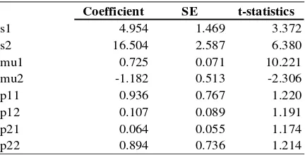
Given the previous conclusion that the data exhibit a two states characteristic, we now present the regression parameters. As can be seen in Table 4, only half of the estimated parameters are statistically significant at 1-percent level (the mean-variance part). The transition matrix is not significant at the standard significance level (95 and 99 percent).
Despite the transition matrix insignificance, the broad interpretation of the model remains appealing. The model suggests that we can divide the JCI into two regimes. State 1 exhibits a positive rate of return (at 0.73 percent per week, equivalent to a 38 percent annualized rate of return). In contrast, state 2 is associated with 1.18 percent weekly loss (61.5 percent annual loss).
The difference between State 1 and State 2 also extend to the volatility side. Variance in the second regime is at 16.5 while in the first regime variance is at 5.0. Hence, in terms of standard deviation, the second regime is 82 percent higher than standard deviation in the first regime.
Table 4. Estimation results of the two states, regime-switching model. Only half of the parameters estimated in the two-state regime-switching model are statistically significant.
Coefficient SE t-statistics
s1 4.954 1.469 3.372
s2 16.504 2.587 6.380 mu1 0.725 0.071 10.221 mu2 -1.182 0.513 -2.306 p11 0.936 0.767 1.220 p12 0.107 0.089 1.191 p21 0.064 0.055 1.174 p22 0.894 0.736 1.214
Source: model calculation.
Thus the first regime is characterized by positive return with low volatilities (and hence, lower risk), while second regime is characterized by negative return, high volatilities/risk.
Despite the statistical insignificance, it is useful to see what the transition matrix imply. The coefficient of the transition matrix shows that State 1 has a probability of 93.6 percent, although there is a 6.4 chance that State 1 may evolve / jump into State 2 in the following period. State 2 has a probability of 89.4 percent, with 10.6 percent chance that it may evolve and move into State 1 in the next period. Given the size of the probability, we may conclude that State 1 is the dominant regime in our period of observation.
Using information from the transition matrix we may calculate the length of each regime. The calculation of the average length of each regime is given by (Wang 2003).
16 6 . 15 9360 . 0 1
1 1
1
11
= = −
=
−p
(12)
Table 3. Log-likelihood, Akaike Information Criteria, and Likelihood Ratio test for various number of states. We compare the AIC for models having 2, 3, 4, 5, and 6 states. Model with 2 states gives the lowest AIC. The Likelihood Ratio tests confirm that, with the exception of model with four states, all models are equivalent
Number
of States Switching Types
- Log Likelihood
Number of
Parameters AIC LR Test df
2 Mean and Variance -1008.394 8 3.814 18.795 40
3 Mean and Variance -1004.958 15 3.827 11.922 33
4 Mean and Variance -1078.761 24 4.138 159.528 24
5 Mean and Variance -1000.280 35 3.885 2.566 13
6 Mean and Variance -998.997 48 3.929 na na
Source: model calculation.
From this formula we can infer that State 1 has an average length of 15.6 periods (16 weeks, roughly 4 months), while the State 2 has an average length of 9.4 periods (9 weeks, roughly two and half months). Since the parameters in the transition matrix are estimated with errors, consequently the length of the first and the second regime can vary as well. Care must be taken, however, in using these numbers, given the wide errors in estimating the transition matrix.
The result from the estimation can also be used to divide the historical data into several periods. This is shown in Figure 3.
Source: own calculation
Figure 3. Evolution of states in the IDX for the entire data (15 January 2000 – 7 September 2007).
Source: own calculation.
Figure 4. Evolution of states in the IDX for the last 50 weekly data (23 September 2006 – 7 September 2007). The final seven observations, from 28 July 2007 until 8September 2007,are in the second regime. Prior to that (from 3 February 2007 until 21 July 2007, 25 weeks) the market was in the first regime.
The figure 3 confirms what we have learned this far, that the length of the State 1 is, on average, longer than the State 2. Further, at the end of our sample period, the probability of being in State 1 is slightly lower (at 0.4437, compared to 0.5563 in State 2) hence we categorized the final data as belonging to State 2.
Discussion
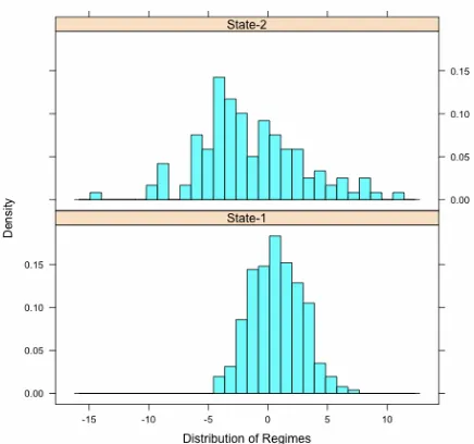
The regime switching calculation performed earlier neatly classifies the market condition into two states. It is tempting to label these states as bullish-bearish regime. This classification is appealing because the market situation is couched in terms accepted by many market participants. However, for the IDX data that are being analyzed, such labeling is not entirely correct because in reality the major difference between the regimes lies in terms of volatility (ie. variance). The difference between the mean of the two regimes (0.712 in state 1 versus 1-.1.182 in state 2) are not statistically significant especially because the standard deviation of the mean in state 2 is quite big (0.513).
In contrast, the difference between variances in the two regimes is statistically significant. Hence, for practical purpose, the defining characteristics between the two regimes are the volatilities. Therefore, despite the two-regime characters, the appropriate description is not the traditional bulls vs. bears, but rather stable versus volatile. This is clearly shown in Figure 5.
Source: own calculation
Our result differs from the result of Turner, Startz, and Nelson (1989), and Maheu and McCurdy (2000). In the latter papers, the bull market (positive return with low volatility) can be contrasted with the bear market (negative return with high volatility). Perhaps one factor that explains the difference is the periodicity of the data. Our estimation uses weekly data for a relatively short period of time, while both the Turner, Startz, and Nelson (1989), and Maheu and McCurdy (2000) use monthly data with windows ranging from 43 to 160 years of data.
The advantage of this paper, however, lies in the fact that information can be adjusted much more frequently on a weekly base (compared to monthly revision). The frequent updating is needed by market players and characterized the behaviour of the retail investors in the Indonesia Stock Exchange.
One important piece of information that can be calculated weekly from the model is the latest probability for each state. We have mentioned previously: “at the end of our sample period, the probability of being in State 1 is slightly lower (at 0.4437, compared to 0.5563 in State 2).” Therefore, since the probability of State 2 has been decreasing, there is an even greater likelihood that the market will move to State 1 (stable state) in the following weeks. In this sense, the usefulness of our calculation result as an early warning signals (EWS) to retail investors becomes clear.
CONCLUSION
Using the regime-switching methodology, this paper confirms that the weekly Indonesia Stock Exchange Data in the period of 15 January 2000 - 7 September 2007 can be characterized by two states. Those states are Stable and Volatile, because the differences of the mean in the two states are not statistically different one from the other. This study also find that the length of the Stable state is 16 weeks on average, while the length of the Volatile state is 10 weeks on average.
For market players, the implications of this research are several folds. First, many local players are short-term traders that thrive on market volatility. For those short-term traders, the model estimated in this paper is useful. Knowledge of the market regime (including the early warning capability of the regime-switching mode) enables these players to time their market activities. Second, short-term market players can expect to continue their activities for a period of time since the regimes usually lasted weeks. The beginning and the end of each regime can also be calculated by feeding updated weekly return data to the already calculated model. Third, the regime switching estimation in this paper is done using
the Indonesia Stock Exchange Index. The same calculation can be done on different data sets (ie. individual stocks). It is possible that different stock may have regimes that do not coincide with the market index movements. Hence market players can sell stocks that enter a stable regime and enter (buy) other stocks that are entering a volatile regime.
While the regime-switching model estimated in this paper has yielded several results important for investment practice, this paper can be extended in several directions. First, we need to check the stability of the coefficients obtained in this paper by doing estimation on different time periods. Second, multivariate models (which include variables such as stock index in other markets in Asia, Europe, or the US) can be considered as additional variables. Movements in the Rupiah/US Dollar can be included in these models as well. In fact, building a multivariate regime-switching model will result in a better early warning signal (EWS).
REFERENCES
Abiad, A. 2003 Early Warning Systems: A Survey
and a Regime-Switching Approach. Interna-tional Monetary Fund.
Alvarez-Plata, P. & Schrooten, M. 2003 The
Argen-tinean Currency Crisis: A Markov-Switching Model Estimation. DIW Berlin, German Institute for Economic Research.
Arias, G. & Erlandsson, U. 2004 Regime switching
as an alternative early warning system of currency crises - an application to South-East
Asia. Lund University, Department of
Econo-mics.
Berg, A., Borensztein, E. & Patillo, C. 2005 “Assessing Early Warning Systems: How
Have They Worked in Practice”? IMF Staff
Papers, 52.
Brooks, C. 2008 Introductory Econometrics for
Finance, Cambridge University Press.
Buckle, R. A., Haugh, D. & Thomson, P. 2002 Growth and volatility regime switching models for New Zealand GDP data. New Zealand Treasury.
Exchange, I. S. 2010 IDX Fact Book, Jakarta,
Indo-nesia Stock Exchange.
Goldfeld, S. M. & Quandt, R. E. 1973 “A Markov
model for switching regressions”. Journal of
Econometrics, 1, 3-15.
Hamilton, J. D. 1989 “A New Approach to the Economic Analysis of Nonstationary Time
Series and the Business Cycle”.
Hamilton, J. D. 1990 “Analysis of time series subject
to changes in regime”. Journal of
Econo-metrics, 45, 39-70.
Kim, C.-J. & Nelson, C. R. 1999 State-space models
with regime switching: classical and Gibbs-sampling approaches with applications, Cambridge, Mass. London, MIT Press.
Kumah, F. Y. 2007 A Markov-Switching Approach
to Measuring Exchange Market Pressure. International Monetary Fund.
Maheu, J. M. & Mccurdy, T. H. 2000 Identifying Bull and Bear Markets in Stock Returns. Journal of Business & Economic Statistics, 18, 100-112.
Mizrach, B. & Watkins, J. 1998 A Markov
Switch-ing Cookbook. Rutgers University, Depart-ment of Economics.
Moerman, G. A., Ers, F. & Revision, A. 2001 Unpredictable After All? A short note on exchange rate predictability. Erasmus Research Institute of Management (ERIM), ERIM is the joint research institute of the Rotterdam School of Management, Erasmus University and the Erasmus School of Economics (ESE) at Erasmus Uni.
Piger, J. 2009 Econometrics: Models of Regime
Changes. Encyclopedia of Complexity and
Systems Science.
Ryden, T., Terasvirta, T. & Asbrink, S. 1996 Stylized Facts of Daily Return Series and the Hidden Markov Model. Stockholm School of Economics.
Turner, C. M., Startz, R. & Nelson, C. R. 1989 “A Markov model of heteroskedasticity, risk,
and learning in the stock market”. Journal
of Financial Economics, 25, 3-22.
Van Norden, S. 1995 Regime Switching as a Test
for Exchange Rate Bubbles. EconWPA.
Van Norden, S. & Schaller, H. 1995 Regime
Switching in Stock Market Returns. Econ WPA.
Van Norden, S. & Vigfusson, R. 1998 Avoiding the Pitfalls: Can Regime-Switching Tests Reliably
Detect Bubbles? Studies in Nonlinear
Dyna-mics & Econometrics, 3.
Wang, P. 2003 Financial econometrics: methods