We find that machine learning models significantly improve the performance of various variables in predicting stock returns. In a recent study, [18] first applies machine learning models to the forecast of stock returns using 94 stock characteristics.
Statistical significance evaluation
Economic significance evaluation
Predictors
Based on different horizons, we have a total of 127 technical indicators.6 To examine whether combining the two sets of predictors could improve forecast power, we use all variables as our third set of predictors. To ensure a robust result, we test not only the statistical significance of different machine learning models, but also their economic significance.
Statistical analysis
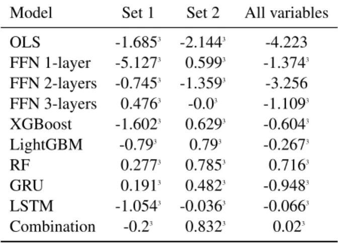
Comparing different sets of predictors, we see that training on 127 technical indicators provides the highest R2OS value in most cases and most models with positive R2OS values (6 out of 9 models). Overall, the results highlight the advantage of using technical indicators in a machine learning model to predict future stock returns.
Portfolio analysis
Therefore, there is much stronger empirical evidence for machine learning models outperforming OLS for training on 127 technical indicators. Therefore, there is stronger empirical evidence for machine learning models outperforming OLS for training on 127 technical indicators.
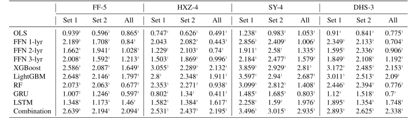
Alpha of bond portfolios
The magnitude of the intercept values is also significantly higher than for training on 94 population characteristics. The results suggest that many returns of H-L portfolios cannot be explained by standard risk factors. The t-test statistic correctly rejects the null hypothesis that the intercepts are zero for all occurrences of training on all 221 variables and 127 technical indicators.
For training on 94 stock characteristics, 3 intercept values are statistically significant at 5%, 1 intercept value is statistically significant at 10%, 1 is not even statistically significant at 10%, while the rest are statistically significant at 1%.
Cross-sectional regression analysis
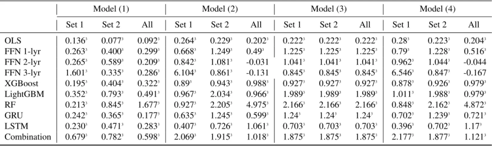
As can be seen, for training on 127 technical indicators and 94 stock characteristics, all thez1 are mostly positive and significant for regression in all 6 regression models. For training on all 221 variables, z1 are negative and not statistically significant for regression in Model (4) and Model (6) for 2-layer FFN and 3-layer FFN. However, it can be seen that the coefficient sizes for training on 127 technical indicators are significantly higher than for training on all 221 variables and 94 stock characteristics respectively.
Therefore, there is much stronger empirical evidence that the independent variables have predictive power for future stock returns cross-training over 127 technical indicators. It can also be seen that the coefficients for the machine learning models are significantly higher than those for OLS.
Economic gains
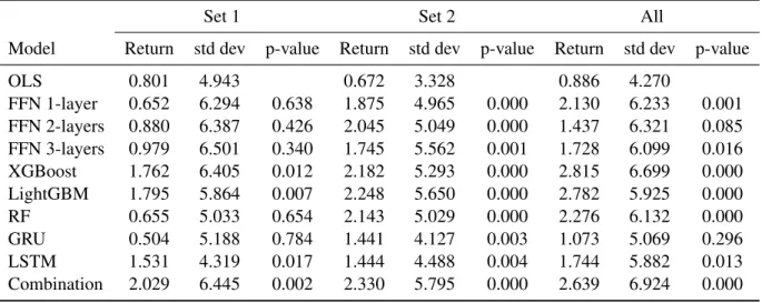
For models trained on 127 technical indicators, all machine learning models have significantly higher Sharpe ratio vs. OLS at 0.202. For models trained on all 221 variables, all machine learning models except 2-layer FFN and GRU have significantly higher Sharpe ratio versus OLS at 0.208. Therefore, there is stronger empirical evidence that machine learning models outperform OLS when they are trained on only 127 technical indicators.
The Sharpe ratios for models trained on 127 technical indicators are significantly higher than those for models trained on 94 stock characteristics. For Sharpe ratio metric, there is weak empirical evidence for machine learning models outperforming OLS when trained on 94 stock characteristics. For models trained on 127 technical indicators, 5 out of 9 ML models (FFN 1-layer, FFN 2-layer, FFN 3-layer, Random Forest and GRU) significantly outperform OLS.
It can also be seen that models trained on 121 technical indicators have much lower maximum draws than models trained on all 221 variables and 94 stock characteristics, respectively.
Transaction cost analysis
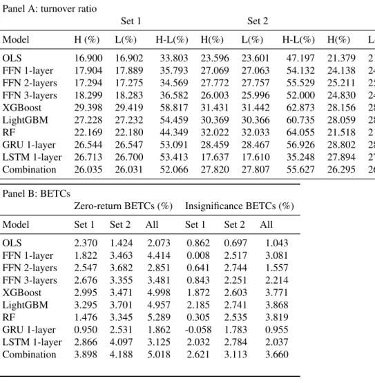
Although some learning models are unable to outperform OLS for maximum moves, in the long run machine learning models can escape the volatility and outperform OLS. Consistent with previous sections, it can be seen that the zero-return BETCs for models trained on 127 technical indicators are significantly higher than for models trained on 94 stock characteristics. We will now discuss insignificant BETCs (transaction costs to make H-L returns statistically insignificant at the 5% level).
For the OLS model, the insignificant BETC is 0.862% for the model trained on 94 stock characteristics, 0.697% for the model trained on 127 technical indicators, and 1.043% for the model trained on all 221 variables. For models trained on 94 stock features, only XGBoost, LightGBM, LSTM, and Combination significantly outperform OLS. Therefore, for zero returns and insignificant BETCs, there is strong empirical evidence for machine learning models outperforming OLS for training on all 221 variables and 127 technical indicators, respectively.
These figures are higher than 0.48%, which is the average round-trip transaction cost for a medium-sized corporate bond trade, estimated by [15], or 0.89%, estimated by [5].
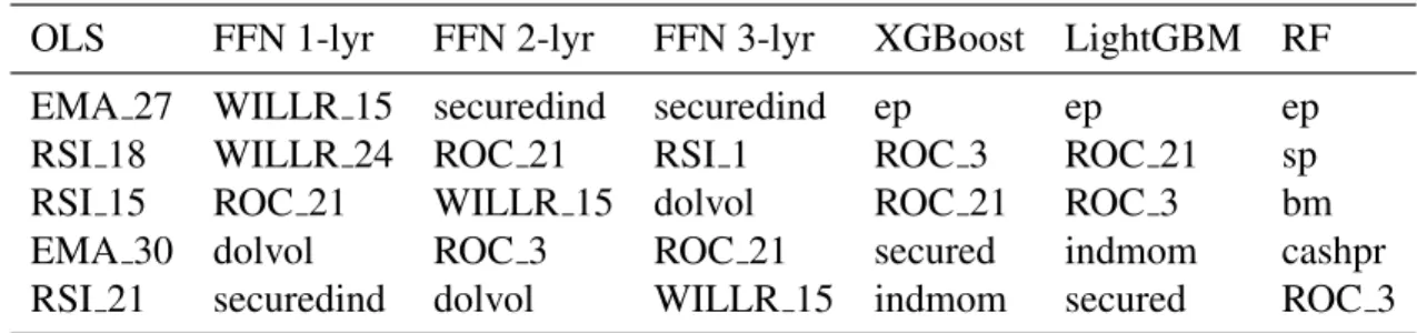
Variable Importance
We use technical indicators such as Simple Moving Average (SMA), Exponential Moving Average (EMA), Average True Range (ATR), Relative Strength Index (RSI), Average Directional Index (ADX), Rate of Change (ROC), William%R (WILR), Commodity Channel Index (CCI), Price Volume Trend (PVT) and Chaikin Money Flow (CMF). Relative Strength Index, Rate of Change (ROC), William%R (WILLR) and Commodity Channel Index (CCI) are momentum indicators. These are followed by the 15-month lag William %R (WILLR 15), the secured debt indicator (securedind), the dollar volume traded (dolvol), and the price-to-earnings ratio (ep), which appear in 3 of the 7 models.
21 months lag Rate of Change, 3 months lag Rate of Change, 15 months lag William %R are momentum indicators.
Interaction effects
The minimum value (expected return) of the quintile 1 curve is also much lower than the minimum value of the quintile 5 curve. For Industry Momentum, the quintile 1 and quintile 5 curves have approximately the same downward-sloping curves. For secured debt, the curve for quintile 1 overlaps strongly with that of quintiles 2, 3 and 4, while the curve for quintile 5 is quite distinct from the other curves.
For earnings to price, the quintile 1 curve has a downward-sloping polynomial shape, while the quintile 5 curve has a roughly downward-sloping exponential shape. For Industry Momentum, the quintile 1 curve has a roughly downward sloping linear shape, while the quintile 5 curve is relatively flat. For dollar revenue volume, the quintile 5 curve is very close to the quintile 4 and quintile 3 curves, while the quintile 1 curve is very distinct from the other curves.
For dollar trading volume, the curve of quintile 1 is roughly bowl-shaped, while the curve of quintile 5 initially has a downward slope shape, which then flattens out at quintile 2 of WILLR 15.
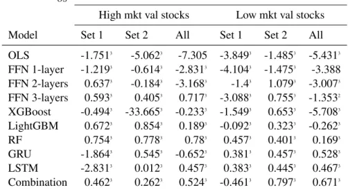
High and low market value stocks
However, this time, 5 out of 9 models significantly outperform OLS for training on 94 stock characteristics (with 4 models statistically significant at 1%). Panel C of Table 10 reports the alphas of the time series regressions of portfolio excess returns in the factor model, (5) Stambaugh and Yuan (2016) mispricing factor model (SY-4). It can be seen that for stocks with high market value, alphas are positive and statistically significant, while for stocks with low market value, alphas are mostly not statistically significant.
Finally, Panel D of Table 10 reports the results of cross-sectional Fama-MacBeth regressions on the following stock characteristics; (6) dividend to price, earnings to price, sales to price, cash flow to price ratio, MAt−1.6, MAt−1.48, MAt−1.6ret, MArett−1.48, return volatility , earnings volatility, return on assets, return on equity and return on invested capital. Z1 are generally positive and statistically significant for both high value and low market value stocks. Since [18] did not consider RNN, GRU and LSTM in their paper, we will not consider the models here.
Due to computational cost, we will not train deep learning models namely Recurrent Neural Network, Gated Recurrent Unit and Long Short Term Memory here.
Alternative tuning method
By considering more hyperparameter combinations when training machine learning models, we are more likely to reach the global optimal outcome and improve prediction performance. Similar to the results using our tuning method, the highest R2OS values are observed for machine learning models trained on 127 technical indicators. Therefore, we will focus our comparison discussion on using 127 technical indicators as predictors.
As can be seen for FFN 2-layer and FFN 3-layer, our method outperforms using the alternative tuning method. As can be seen, for some models of FFN 1-layer, FFN 2-layer and FFN 3-layer, when trained using the alternative tuning method, their average returns are significantly lower than those of models trained using our tuning method. For LightGBM and XGBoost, the average return for training on all 221 variables using our tuning method is significantly higher than using the alternative tuning.
Therefore, it is recommended to adopt our much wider range of hyperparameters setting for FFN 1-layer, FFN 2-layer, FFN 3-layer, LightGBM and XGBoost, even if it is computationally more expensive.
Empirical results for rolling training process
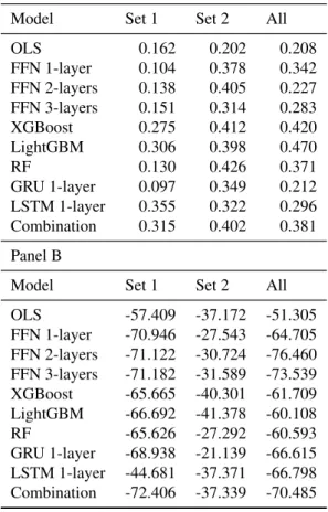
As can be seen, most of the R2OS results are significantly better than previous results using a fixed training process (training on the first 240 months of data). As can be seen, most of the average regression results are significantly better than the previous results using a fixed training process. This table reports the proportional reduction in mean squared prediction error (R2OS) for different predictive models (linear predictive model or machine learning models) that use three sets of predictors v.s.
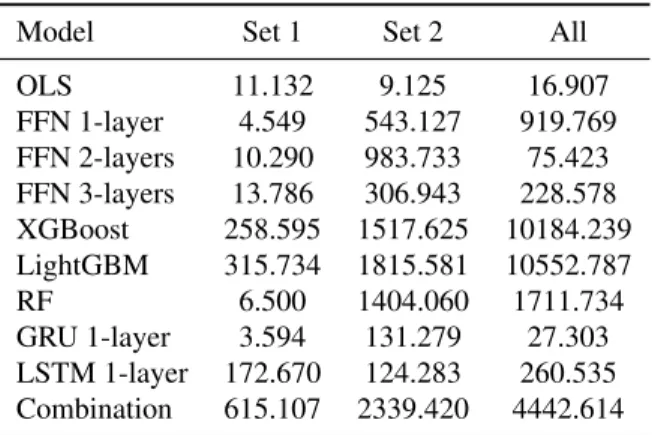
This table reports the returns of zero-investment portfolios ranked by expected stock returns over the one-month holding horizon. This table reports the cumulative returns of zero-investment portfolios over the test period. This table reports the results of cross-sectional regressions of individual stock monthly returns on expected return predicted by all 221 variables, 127 technical indicators and 94 stock characteristics variables respectively.
Panel A reports the proportional reduction in root mean square forecast error (R2OS) for different predictive models (the linear predictive model or machine learning models) using three sets of predictions vs. Panel B reports the return and p-value for the two-sample t-test with the null hypothesis (H0) being:RML−RLR≤0, where RMLi is the return of the null investment portfolio from the machine learning models and RLR denotes the return from the linear predictive model. Panel B reports returns, standard deviation of returns, and two examples of t-tests for excess return dispersion of decile-sorted portfolios sorted by stocks' expected returns for all stocks.