Resource management technical reports Natural resources research
2006
Potential impacts of climate change on agricultural land use Potential impacts of climate change on agricultural land use suitability : canola
suitability : canola
Luke Vernon Dennis Van Gool
Follow this and additional works at: https://researchlibrary.agric.wa.gov.au/rmtr
Recommended Citation Recommended Citation
Vernon, L, and Van Gool, D. (2006), Potential impacts of climate change on agricultural land use suitability : canola. Department of Primary Industries and Regional Development, Western Australia, Perth. Report 303.
RESOURCE MANAGEMENT TECHNICAL REPORT 303
CLIMATE CHANGE ON
AGRICULTURAL LAND USE SUITABILITY:
CANOLA
Luke Vernon and Dennis van Gool
March 2006
Resource Management Technical Report 303
Potential impacts of climate change on agricultural land use suitability:
Canola
Luke Vernon and Dennis van Gool
March 2006
Disclaimer:
The Chief Executive Officer of the Department of Agriculture and the State of Western Australia accept no liability whatsoever by reason of negligence or otherwise arising from the use or release of this information or any part of it.
Summary
A relatively simple model was developed to generate climate change scenarios for a variety of agricultural crops. The model was only partially validated against real data, hence it is best used as a decision support system that allows people with land resource, crop and climate knowledge to determine potential impacts of climate change on crop growth and production.
Land use capability data and climate information for the agricultural zone of Western
Australia were combined with a modified French and Schultz equation to produce a potential yield map for canola. Another yield map was then produced for 2050 based on SRES
marker scenario A2, CSIRO Mark II, which is considered a good model for the South West of Western Australia.
Climate change in WA may result in relatively large reductions (>30 per cent) in canola yield potential in the northern agricultural region (around Mullewa) by 2050 due to reduced rainfall and higher maximum temperatures. Current production is not very high in the northern agriculture region. Of the major growing areas, Gnowangerup, Lake Grace, Jerramungup and Esperance stand out as likely to experience significant reductions in yield.
The CSIRO model predicts a small increase in both maximum and minimum temperatures, of around 0.8 degrees Celsius. Both the year 2050 temperature prediction and the crop
response to temperature are uncertain. High temperatures will reduce soil moisture, change disease risk and have direct effects on growth. We believe a high temperature effect is likely, though the amount of the actual temperature increase and the effect on canola yield is uncertain. It is possible that the high temperature effect on canola growth is offset by
increased CO2 levels, which are not considered in our model. The effect of minimum temperature on canola growth was not factored into this model because when a minimum temperature restriction was used it resulted in an underestimation of yield compared to actual yield data for a number of shires.
The model predicts that an extensive area encompassing much of the eastern, central, southern and south-eastern wheatbelt may experience a 10-30 per cent yield reduction by 2050 mainly due to reduced rainfall.
There is a large area where little change is anticipated in the western area of the agricultural zone. However, within this region it is likely that low lying areas perform better as reduced rainfall results in less waterlogging, but drier areas are likely to lose some production.
Overall, this modelling found that 45 per cent of the agricultural zone may experience a decrease in yield potential greater than 10 per cent as a result of climate change. The actual reduction will be less as farmers adapt their planting strategies and canola cultivars.
The model is independent of economic analysis. Our use of the term ‘yield potential’ is indicative, since farmer adaptation occurs anyway and it is difficult to predict how much flexibility there is in this adaptation. This decision support system shows areas of risk, where the capacity to adapt may be strained, e.g. in the northern agricultural region around Mullewa and Mingenew. It also identifies the best places to grow canola in 2050. Examples of
adaptation include the development of new cultivars, such as short season varieties, improvements in management or alternative crops.
Contents
Introduction ... 4
Climatic requirements and Influences ... 6
Soil requirements and influences ... 6
Model development ... 7
Materials and methods... 8
The data ... 8
Software ... 8
Method... 8
Climate change... 17
Model assumptions... 17
Mean values and the French and Schultz equation ... 17
Temperature-related assumptions... 18
Results ... 20
Discussion... 24
Climate change predictions ... 24
Model improvements ... 25
Economic implications ... 25
Future opportunities... 28
Conclusion ... 29
References... 30
Appendix 1: Soil conditions affecting canola... 33
Appendix 2: Canola capability and land qualities... 34
Appendix 3: Selection of temperature limitations... 36
Acknowledgements
The helpful comments of Ron McTaggart of the Department of Agriculture are gratefully acknowledged.
Funding for this work was provided by the Australian Greenhouse Office.
Introduction
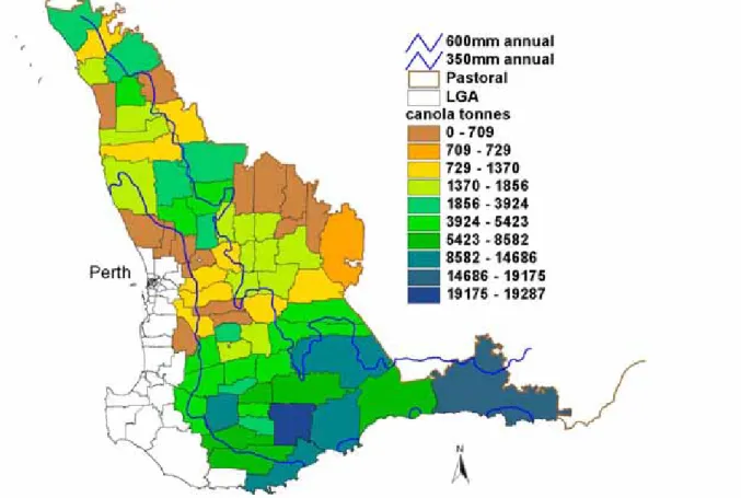
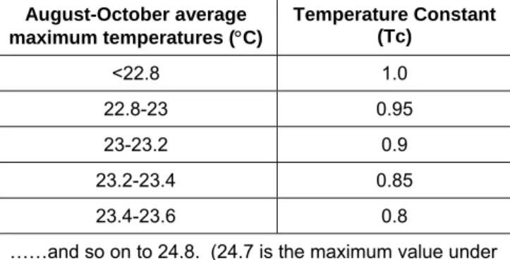
Canola (Brassica napus) was one of the fastest expanding broadscale crops in Western Australia in the 1990s (Carmody and Walton 1998), increasing from approximately 30,000 ha in 1993 (Zaheer et al. 1999) to over 800,000 ha in 2000 (ABS 2005). The area sown has since fallen and in 2004, 420,000 ha was planted (Garlinge 2005). Canola was traditionally grown in areas receiving more than 450 mm average annual rainfall (Carmody and Walton 1998), however, is now grown in areas with an average rainfall as low as 350 mm (Figure 1), due to the development of short season varieties (Garlinge 2005).
Figure 1: Average total canola production (tonnes) for each local government authority for 1995-1999 based on CBH grain receivals
Canola, which is a low erucic acid, low glucosinolate variety of rapeseed (Carmody and Walton 1998), was originally cultivated by ancient civilisations where its oil was used for lighting. It was first grown in Canada as a lubricant in ships (Colton and Potter 1999) and is now primarily used for vegetable oil, which is suitable for many applications such as
margarine, shortening and cooking oils (Garlinge 2005).
Oil concentrations are important to economic returns and can be influenced by cultivar and environment. By and large, canola is regarded as being less tolerant to water deficit that other grain crops (Walton et al. 1999). High temperatures and low soil moisture during pod development can reduce oil concentration by 3-5 per cent (Garlinge 2005).
Climate variability presents a significant challenge to cropping. Records show that rainfall has declined in the South-West, undergoing a sharp and sudden decrease since the 1970s (IOCI 2002). Day and night-time temperatures, particularly in winter and autumn, have
absence of human influence, the changes experienced do not appear to have been caused exclusively by natural climate variability (Sturman and Tapper 1996, IOCI 2002).
In order for the cropping industry to adapt to future variability, it is important to identify likely impacts of climate change. This study aimed to assess how current climate change
scenarios in the agricultural zone will impact on canola suitability and growth. This will help identify areas where future management and research efforts should be focused.
Climatic requirements and influences
The most important climatic factors determining yield and oil concentration are rainfall and temperature (Walton et al. 1999a, Si and Walton 2004). Yield and oil concentration have been shown to increase with increasing post-anthesis rainfall. Si and Walton (2004) found that the rate of increase of oil was 0.7 per cent for every 10 mm increase in rainfall after anthesis and seed yield increased at a rate of 116 kg/ha for every 10 mm increase in rainfall.
Walton et al. (1999b) reported a trend of increased oil and yield in locations with higher rainfall and cooler temperatures after flowering. Thus, the highest yields are often obtained in the medium and high rainfall zones where the growing season is longer (Garlinge 2005).
The optimum temperature for canola is between 20 and 25°C (Carmody and Walton 1998).
Temperatures above 32°C during flowering can cause flower abortion, as can severe frosts at this time. Low temperatures can delay seedling emergence (Carmody and Walton 1998).
High temperatures during post-anthesis reduce oil content and seed yield. Si and Walton (2004) showed that the average rate of reduction of oil content was 0.68 per cent and 289 kg/ha for seed yield for every 1°C increase in post-anthesis temperature. Others have found the rate of decrease of oil content to be as large as 1.5 per cent for each 1°C rise (Hocking and Stapper 1993).
The onset of drought after anthesis has been shown to significantly reduce yield (Richards and Thurling 1978). Si and Walton (2004) commented that increasing heat and terminal spring drought in low rainfall areas have a detrimental effect on yield and oil concentrations.
For many years canola has been predominantly grown in the high rainfall areas (>450 mm annual rainfall) with a long growing season (Si and Walton 2004). However, the release of short season varieties has enabled cultivation in the medium and low rainfall zones, but oil concentration and yields are usually low and variable (Si and Walton 2004).
Soil requirements and influences
Canola can be grown on a wide range of soil types (Garlinge 2005). In general, high yields are obtained on well to moderately well drained soils that have no extremes in pH, are non- saline, have soil water storage of at least 70 mm within the root zone, and a good supply of nitrogen and phosphorus (Carmody and Walton 1998).
One of the major factors affecting canola, particularly in the high rainfall areas of WA, is waterlogging (Walton et al. 1999a). Although the impact can be less severe than on wheat (Zhang et al. 2004), waterlogging can restrict canola yield by up to 50 per cent when compared to a well drained site (Walton et al. 1999a).
Canola is also susceptible to sandblasting from wind erosion during the first four to six weeks (Carmody and Walton 1998). It is slightly tolerant of soil salinity and yield is only affected when ECe >400 mS/m (Carmody and Walton 1998; Walton et al. 1999a).
For further information on soil factors affecting the productivity of canola, refer to the summary in Appendix 1 by Carmody and Walton (1998).
Model development
To estimate yield, the model described in this study uses the rainfall-driven French and Schultz (1984) equation, to which adjustments are made to take into account land capability, waterlogging and maximum and minimum temperatures.
The French and Schultz equation has been accepted as a useful model for grain crops in WA, even though reporting has been informal or anecdotal (e.g. Tennant 2001, Hall 2002).
Some detailed work has been undertaken for grain legumes (Siddique et al. 2001).
The model as reported here was first developed in conjunction with Peter White for use with pulses and legumes in WA and was described by van Gool et al. (2004a,b).
When our yield predictions seem reasonable, the effects caused by climate change are predicted by rerunning the model for a selected 2050 climate scenario.
The model is a good tool for combining complex data and expert knowledge. It bridges the gap between a number of scientific disciplines and several audiences, including:
• People involved in planning and policy
• Land users and managers, including research agronomists, technicians and farmers.
Materials and methods
The data
• Bureau of Meteorology (BoM) climate surfaces for rainfall, maximum temperature and minimum temperature. These are mean daily values for each month for 1961 to 1990 shown on 0.25 x 0.25 degree grid cells (approx. 2.5 km).
• Department of Agriculture’s map unit database and land resource maps to create land capability maps for each crop. Mapping scales range from 1:20,000 to
1:250,000. See Schoknecht et al. (2004) for an overview of soil-landscape mapping methods and outputs and van Gool et al. (2005) for an explanation of land qualities and land capability.
• Ozclim climate scenario (SRES Mark II) available from CSIRO Atmospheric Research which predicts changes in rainfall plus maximum and minimum temperature.
• BoM Patched Point climate data.
• Published and unpublished information about the crops.
• CBH Grain bin receivals information for 1995 to 1999 summarised for local
government areas prepared by the Farm Business Development Unit, Department of Agriculture.
Software
The mapped information was prepared using Arcview 3.2 and Spatial Analyst. The gridded BoM climate and Ozclim climate change information was matched to the centroid of each soil-landscape map unit by a unique identifier. Only matching grid cells were used and no attempt was made to summarise further. The information was then exported to an Access 97 database, where all the yield calculations were done. The information was then exported back to Arcview for display, but any other GIS package could be used.
Method
Yield
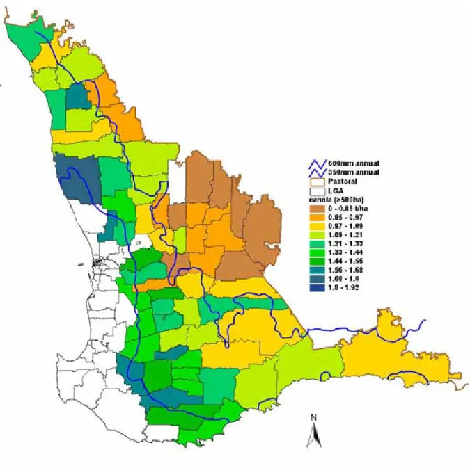
Initial estimates of water use efficiency were derived from the literature. After a review by staff from the Australian Greenhouse Office it was requested that this information be scaled to real data. We had mean values for yields based on CBH grain receivals (Figure 2) and corresponding BoM rainfall records 1995-1999 readily available.
The grain receival figures give more conservative estimates of water use efficiency than others (e.g. French and Schultz 1984, Tennant 2001, Hall 2002). The yields represent averages achievable in the south west agricultural region in 1999. It should be noted that the mean yields are then scaled both up and down for good and poor cropping land as indicated by the land capability which considers both the soil type and the position in the landscape.
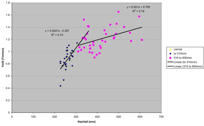
Figure 2: Mean canola yields (tonnes/hectare) 1995-1999 based on CBH grain receivals To analyse the CBH figures, in the interests of simplicity, and because there was insufficient data to warrant using a more complex model, the equation was partitioned using two linear regressions of yield and rainfall (Figure 3). For 150-310 mm rainfall the regression line is similar to the French and Schultz (1984) equation and for 310-600 mm there is a line showing much lower water use efficiency. The lines were drawn where they best represented the data (the R2 values were maximised). Up to 31 0 mm there was a very good fit of the data. Beyond 310 mm the data fit poorly. The use of two linear regressions instead of a polynomial equation is generally not condoned, however it is a pragmatic solution for our decision support tool. The ‘x’ intercept of the line from 150 to 310 mm was also used to estimate the evaporation water loss (75 mm).
Canola
y = 0.0047x - 0.357 R2 = 0.70
y = 0.001x + 0.795 R2 = 0.19
0 0.2 0.4 0.6 0.8 1 1.2 1.4 1.6 1.8
0 100 200 300 400 500 600 700
Rainfall (mm)
Yield (Tonnes) canola
to 310mm 310 to 600mm Linear (to 310mm) Linear (310 to 600mm)
Figure 3: Linear regressions on mean canola yields 1995-1999 based on CBH grain receivals (scaled to 1999 figures)
Mean yield was estimated using a modified equation of French and Schultz (1984).
Adjustments for excessive rainfall (WAc), soil capability class (LCc), minimum temperature (Mintc), maximum temperature (Maxtc) were added.
[1] (If GR ≤310mm) MY = WUE1 × (GR – WL) × WAc × LCc × Mintc × Maxtc [2] (If GR >310mm) MY = WUE2 × GR + YI × WAc × LCc × Mintc × Maxtc MY = mean yield
WUE1 = water use efficiency which is approximately 4.7 (from CBH grain receivals) WUE2 = water use efficiency which is approximately 1 (from CBH grain receivals) YI = Yield at the intercept of the two regression equations = 1105 kg
GR = growing season rainfall 1 May to 31 October, plus 20% of rainfall 1 November to 30 April (20% accounts for initial soil moisture available to the crop)
WL = water loss
If GR ≥150 mm/yr THEN WL = 75 If GR < 150 mm/yr THEN WL = GR × 0.5 WAc = waterlogging constant (see below)
LCc = land capability class constant (see below) Mintc = minimum temperature constant (see below) Maxtc = maximum temperature constant (see below)
Waterlogging constant (WAc)
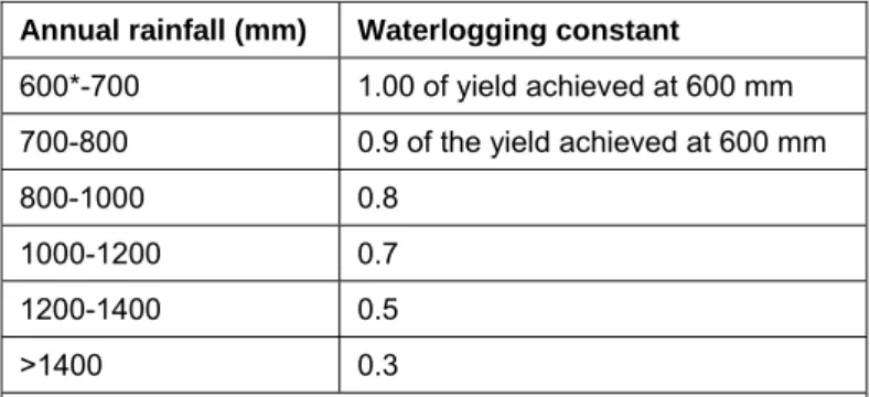
In this scenario growing season rainfall above 310 mm is approximately where the water use efficiency of canola growth declines dramatically for a variety of reasons. Excess water is removed by run-off or leaches beyond the root zone, and increased disease problems can reduce predicted yields. Waterlogging and increased incidence of disease will result in yield
reductions when rainfall becomes very high. In the absence of better data, yield potential was decreased for increasing rainfall above 600 mm (Table 1). Further data were not sought because of time constraints, because it would have only a small impact on our model
because 600 mm occurs near the edge of the State Forest which is a distinct physical boundary for the cropping region. (State Forest areas are shown on Figure 13.) Table 1: Waterlogging constants for adjusting yield potentials for annual rainfall
Annual rainfall (mm) Waterlogging constant
600*-700 1.00 of yield achieved at 600 mm 700-800 0.9 of the yield achieved at 600 mm 800-1000 0.8
1000-1200 0.7 1200-1400 0.5
>1400 0.3
*600 mm occurs near the edge of the State Forest creating a distinct physical cropping region boundary.
Land capability constant (LCc)
'Law of the Maximum' (Wallace and Terry 1998) states that a large yield response is possible if there is only a single limiting factor, but as the capability table indicates (Appendix 2), if one limitation is overcome, others soon come into play. This suggests that only when all limiting factors are addressed simultaneously does plant production have a chance of reaching biological potential. For this reason using land capability maps based on many factors for this yield model we believe is superior to models driven from only one or two more readily available, or better understood properties, such as soil water storage or pH. Lower capability means greater constraints for plant growth and reduced yield, hence the average yield is scaled using the values listed in Table 2.
Table 2: Constants for adjusting yield potentials on each land capability class
Land Capability Class Land Capability Class Constant (LCc)
1 1.8 2 1.4
Higher than average yields
3 1.0 Average yields
4 0.6
5 0.4 Lower than average yields
Land capability ratings for canola were based on van Gool, Tille and Moore (2005), Carmody and Walton (1998) and Maschmedt (unpublished), with fine-tuning in consultation with canola agronomists from the Department of Agriculture. The ratings can be best described as considered judgements taking into account local experience and the research data that was available (both published and unpublished).
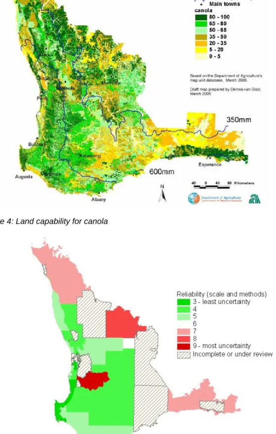
The development of the ratings involved several iterations. Ratings were fine-tuned until there was consensus that the maps of land capability provided a good general representation of reality (see Figure 4) in the context of a subjective evaluation of survey quality using the date of publication, survey methods and the mapping scale (see Figure 5). See Appendix 2 for the final capability table.
Figure 4: Land capability for canola
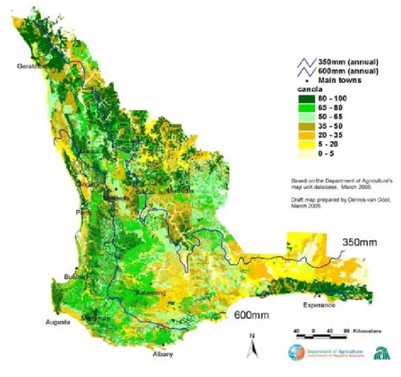
Figure 5: Subjective assessment of reliability based on mapping scale and survey methods
Temperature constants (Mint, Maxt)
Maximum and minimum temperatures for canola growth were collated from Ecocrop (FAO 1996) and the Australian software program PlantGro™ (Hackett 1999). These values suggest that canola experiences significant yield reductions when the temperature exceeds 37°C and may die when temperatures exceed 40°C. At the low temperature extreme, yield is depressed significantly at -3°C and plants normally die at -6°C.
These temperature values were then related to averages of the daily monthly maximum and minimum temperatures on the BoM climate surfaces (see Tables 3 and 4). It should be noted, however, that the minimum temperature restriction for canola was not used in this model because using it produced a poor correlation between modelled yields and actual CBH yield data. See model iterations below for more information.
Because we are using daily temperatures averaged for an entire month there will be a significant fluctuation of temperature around this value, hence the temperatures reported in Tables 3 and 4 may seem higher or lower than expected. Refer to Appendix 3 for how the yield limiting temperature values in Tables 3 and 4 were estimated.
For maximum temperature, the three months August to October were used. During this time there is a fairly linear increase in temperature, and more warm days in October than August.
For minimum temperature, -5°C is rare, but frosts are common in some regions. September was selected because crops are highly vulnerable to frost damage at this time. Our
minimum temperature restriction is loosely related to the likelihood of frosts (see Figures A4 and A5 in Appendix 3).
A maximum temperature was selected using a monthly mean about 13°C less than the point at which significant plant stress was thought to occur. For the minimum temperature, the monthly minimum was about 9°C higher than the point at which significant plant stress was thought to occur. Other than FAO (1996) and Hackett (1999), there was little real data to support these selections in WA. However, the model iterations, discussed below, were used to fine tune the temperature adjustments.
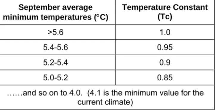
Tables show how yield is decreased as average maximum temperature increases (Table 3) and average minimum temperature decreases (Table 4) below the critical levels. See Appendix 3 for further information on the selection of temperature limitations using monthly averaged data.
Table 3: Temperature constants for adjusting yield potentials for average maximum temperatures (August to October)
August-October average
maximum temperatures (°C) Temperature Constant (Tc)
<22.8 1.0 22.8-23 0.95 23-23.2 0.9 23.2-23.4 0.85 23.4-23.6 0.8
……and so on to 24.8. (24.7 is the maximum value under the 2050 climate scenario)
Table 4: Initial temperature constants for adjusting yield potentials for average minimum temperatures in September
September average
minimum temperatures (°C) Temperature Constant (Tc)
>5.6 1.0 5.4-5.6 0.95 5.2-5.4 0.9 5.0-5.2 0.85
……and so on to 4.0. (4.1 is the minimum value for the current climate)
Note: The minimum temperature constraint was removed from the model during iterations.
Model iterations
As described, considerable effort went into reaching land capability maps that accorded with
‘expert’ opinion. Maps underwent several iterations and the results were discussed until a consensus was reached that they were a reasonable representation of reality.
When yield maps have been prepared the results can be verified against actual yield data.
However, this is complicated by huge diversity in trial information, including the methods adopted for the trial, the reporting methods and the lack of detailed climate and soil information at the trial sites. A visual assessment of the mapped areas indicates that the modelled maps show high yields where existing trials yield well and vice versa. Trials should be considered because it would minimise variability due to management and farm
economics. Trial information yields higher than achievable on most operational farms and is not readily available over extensive areas. Early wheat research trials reported by Davidson and Martin (1968) indicate that farm wheat yields for selected sites in WA achieve between 57 and 72 per cent of experimental yields. The model considers a mean yield based on 1995-1999 CBH yields (Figure 2) as such data were readily available. Because there is a gradual increase in yield over time the CBH figures are scaled to 1999 yields.
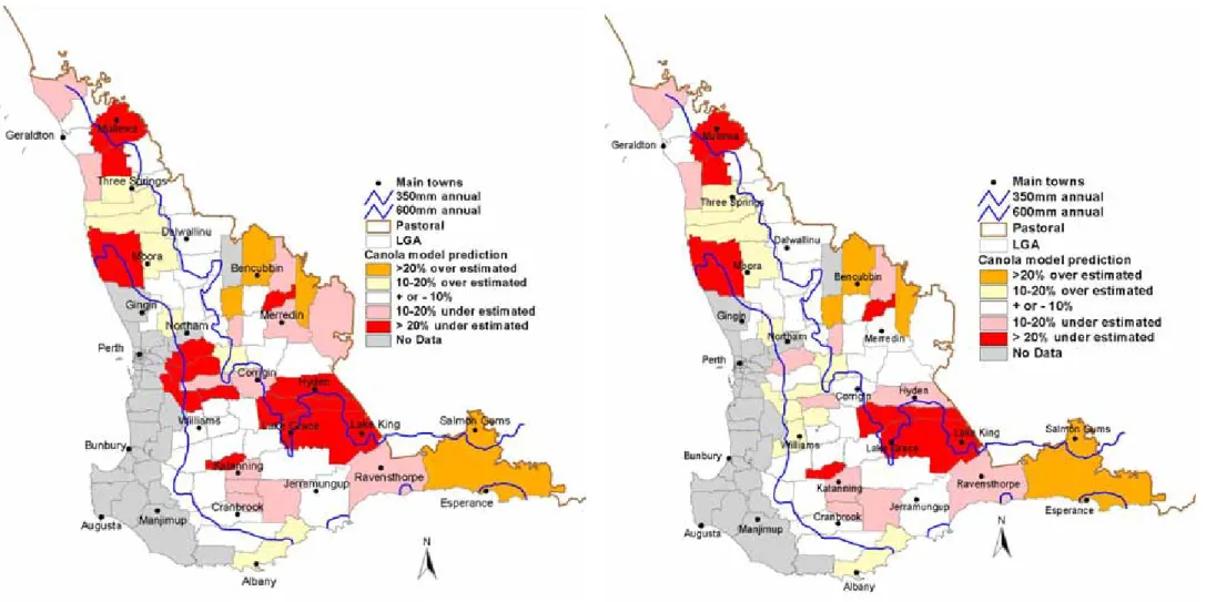
It is instructive to view the comparison of modelled and actual shire yields spatially. Figure 6 shows where the model predictions were out by more than ±10 per cent. The literature (Carmody and Walton 1998) indicates that there may be a yield reduction because of low temperatures and frost damage. However it was noted that several LGAs toward the middle of the map underestimated canola yield because the minimum temperature restriction was too severe. Figure 7 shows a closer correlation of the model to the actual yield data when the minimum temperature restriction was removed.
Figure 6: Areas where model varies from the CBH 1995-99 data by
±10%
Figure 7: Areas where model varies from CBH 1995-99 data by more than ±10% when yield penalties for minimum temperature are removed
Canola has the smallest total yield of all crops studied in this series (wheat, barley, oats and lupins) hence a poor model match in shires which grow little (see Figure 1) might be
expected. However the greater than 20 per cent underestimates north of Jerramungup in important canola growing areas, such as Lake Grace and Kulin are difficult to explain when Esperance is overestimated and Jerramungup is a good match to the model. A number of reasons why it is unreasonable to expect a perfect match of real data to our simple model are discussed below. However it is possible that soils planted to canola within shires are more selective than expected creating a strong bias to the overall capability of all soils in the shire. This would seem unlikely as canola can be successfully grown on a wide range of soil types. It is possible that our land capability maps were more restrictive than expected, as the shires north and east of Jerramungup have a higher proportion of low capability land. It is also worth noting that the reliability of the land capability information is lower here (Figure 5).
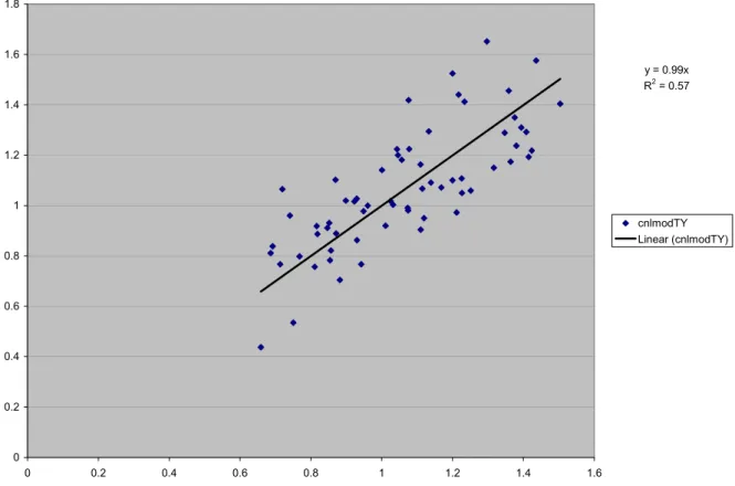
Figure 8a shows yield predicted by the model, averaged for each local government area against CBH yield. Figure 8b shows the yield predicted by the model against ABS crop yield figures for 1983-87 (ABS figures are comparable to CBH figures). A linear regression is not ideal, as CBH yields are not an ideal ‘known’ value and have a significant amount of
variability. There is uncertainty in assessing which locations deliver to particular storage bins. Also some crops do not go via the local storage bins. Even if the yield figures are reliable there is variation in management, varieties, planting times, climate and soil types.
The graph indicates the model has a moderate predictive ability, which is not surprising given the general assumptions made (discussed under model assumptions). Particular attention is drawn to the assumption that all soils in a local government area are considered. It should be remembered that the model attempts to predict where productivity of cropping land for canola is likely to change as a result of climate change, irrespective of whether it is being cropped for canola currently (e.g. Figure 1).
This allows prediction of possible shifts in productive areas. Hence the CBH data are used to scale the information rather than for validating the model.
y = 0.99x R2 = 0.57
0 0.2 0.4 0.6 0.8 1 1.2 1.4 1.6 1.8
0 0.2 0.4 0.6 0.8 1 1.2 1.4 1.6
cnlmodTY Linear (cnlmodTY)
Figure 8a: Modelled versus actual yield for 1995-99 in tonnes
y = 1.03x R2 = 0.23
0 0.2 0.4 0.6 0.8 1 1.2 1.4 1.6 1.8
0 0.2 0.4 0.6 0.8 1 1.2 1.4 1.6
cnlmodTY Linear (cnlmodTY)
Figure 8b: Modelled versus actual yield for 1983-87 in tonnes
Climate change
Climate change scenarios to 2050 were generated using OzClim, which is a climate scenario generator that simplifies the process. OzClim is available from CSIRO Atmospheric
Research (email [email protected] or http://www.dar.csiro.au/publications/ozclim.html).
The temperature change scenario was the SRES A2 CSIRO Mark II. OzClim was used to calculate surfaces that show the difference from the base climate (1961-90). Ozclim values are used to adjust the current base climate values (1961-90) which are at 2.5 km resolution.
This is preferable to using the 25 km resolution surfaces generated from Ozclim directly.
The entire model is then simply re-run for the new climate.
Model assumptions
This model/decision support tool assumes:
Management practices, whether improvements or a result of a response to climate change such as different planting times, do not alter over the course of the scenario.
Carbon dioxide concentrations remain the same. This is important when considering the results, as modelling by Howden et al. (1999) showed that wheat yields would more than likely increase at all sites studied (Geraldton, Wongan Hills and Katanning) under future climate change scenarios with a doubling of current carbon dioxide levels.
Plant growth responses to temperature extremes or excessive rainfall are generally not linear except over a small portion of the response curve, Tables 3 and 4 show a linear
relationship of waterlogging and temperature to growth. This is because the lowest
limitations for canola and the 50 year climate change scenario climatic adjustments are relatively small. Waterlogging/disease limitations apply after 600 mm, but this occurs mostly in forest/water catchment areas (shown on Figure 7) that are not available for cropping. The model would need temperature and waterlogging responses checked for other regions, or if climate change was much greater than presently predicted.
All soils within a local government area are considered. In reality some soils would simply not be cropped e.g. saltland or bare rock. The maps indicate high and low productivity land and show where productive land might be lost as a result of climate change.
Because there is no record of which soils are actually cropped, validating the model against grain yield records based on local government areas can only be indicative.
Because the model considers all land in a local government area, if there is a large
amount of class 5 land the model would predict reduced yield. This would be misleading if canola is only grown in a portion of the shire where class 1 to 3 land dominates. Although canola can be grown on a wide range of soils, there are many shires where only small amounts are grown, which is a potential source of error when scaling the model against shire yield data.
Mean values and the French and Schultz equation
The model deals with average conditions. It does not consider climate extremes (droughts and floods) which are reported to be more frequent with climate change (e.g. IPCC 2001).
The French and Schultz equation is an appropriate tool for dealing with average climate values (e.g. BoM 1961-90). It is not suitable for crop growth in a single season because it only considers if there is adequate rainfall over the growing season. If the rain falls too early or too late in the season there will be a large effect on crop growth that cannot be predicted.
Over a longer period these seasonal differences are averaged out.
Temperature-related assumptions
There is no yield penalty for minimum temperature.
Frosts can reduce yields by damaging plants, but cooler temperatures are beneficial for consistent grain filling, hence the response can be difficult to predict.
The temperature requirements for different cultivars can vary greatly. However, the model assumes a single cultivar for a given scenario.
There are interactions between temperature and moisture availability. For example canola will tolerate 40°C if soil moisture is not limiting and the plant is not under moisture stress.
The temperature/moisture interaction can be built into the model (and has been trialled), but was not used for the scenarios generated for this report.
There are critical temperatures for different stages of crop development. Adding temperature criteria for other months to account for critical plant growth periods would be straight forward.
When it is warmer canola has short grain filling, hence there is less opportunity to achieve good yields, and any moisture or temperature stresses will reduce yields more than in cooler areas. The model assumes a single cultivar, though a new scenario could be generated for each cultivar if the climatic or soil requirements were known to be significantly different.
Temperature may not be a direct problem for the plant, but evaporation and evapo-
transpiration may dry soils out before the crop has finished growing. This was considered when making high temperature selections in the model.
Higher temperatures are generally correlated with increased numbers of plant pathogens.
This was considered when making high temperature selections in the model.
Finding detailed climate information for canola suitable for preparing regional summaries using monthly averaged temperature data proved difficult. It is generally accepted that temperature affects growth and yields. However, we are unaware of any regional temperature modelling that has been quantified, hence our initial predictions are largely based on estimates from the literature and field knowledge from canola agronomists. Model iterations were then used to adjust these values.
Results
Potential canola yield decreased in various magnitudes in the north, south and east of the agricultural zone due to rainfall change only, shown in Figures 9 and 10. Western areas of the agricultural zone had no change in potential yield (Figures 9 and 10).
Changes due to rainfall plus temperature are displayed in Figures 11 and 12 and a difference map is displayed in Figure 13. These show a widespread reduction in the agricultural zone of 10-20 per cent east of a line running from just east of Katanning north to Three Springs.
North of Three Spring larger reductions are predicted, with a 20-30 per cent decrease.
Further north around Mullewa greater than 30 per cent reduction is predicted.
There is a relatively large area of no change in the western wheatbelt east of the State Forest and along the coast in the south and south-eastern wheatbelt (Figure 13).
About 45 per cent of the land, or 12 million hectares showed reduced potential yield of 10 per cent or more. The remaining 14.7 million hectares did not change (i.e. more than ±10 per cent). This was the largest decrease predicted for the crops studied as shown in Table 5.
Table 5: Area experiencing change in potential yield for crops analysed in this study (van Gool and Vernon 2005, van Gool and Vernon 2006, Vernon and van Gool (2006a,b)
Area of agricultural zone experiencing change of potential yield (%)*
Reduction Barley Canola Lupin Oats Wheat(a) Wheat(b)
Large (>30%) 2 1 0 <1 (0.1) 3 2
Moderate
(20-30%) 4 4 <1 (0.3) 1 3
Small (10-20%) 37 40 27 39 36
32
No change
±10%) 57 55 73 60 58 59
(plus 8%
increase) (a) are the updated values when wheat is re-run using the current model (utilising two linear regressions).
(b) are the values published in van Gool and Vernon 2005. Note this model predicts a small area of yield increase because it assumes yield penalties when growing season rainfall exceeds 400 mm. The current model uses 600 mm.
* Total area of the agriculture region is approximately 26.7 million hectares.
Figure 9: Current potential yield based on rainfall Figure 10: 2050 potential yield based on rainfall
Figure 11: Current potential yield based on rainfall and temperature Figure 12: 2050 potential yield based on rainfall and temperature
Figure 13: Canola yield change over 50 year scenario when current potential yield was greater than one quarter of the maximum potential achieved by the model (481 kg/ha). Note: isohyets are current annual rainfall contours
Discussion
The large decrease (more than 30 per cent) in potential yield in the northern wheatbelt is due to a combination of high temperatures and change in rainfall over 50 years.
Temperature change is less reliably predicted by climate scenarios, and the specific impact of high temperature on canola yield is subject to debate. Further uncertainty is cast by modelling by Howden et al. (1999), which indicated that under a doubling of CO2
concentrations, wheat (hence canola) yields might actually increase with climate change. It should be noted that in our generic model high temperature effects are based on grain yield, and not dry matter production. High temperatures will reduce soil moisture stores more rapidly, and increase the likelihood of some diseases, as well as impact directly on canola growth. With temperature, the main effect is a shorter growing season. Development of short season varieties could potentially offset yield reductions more than reduced rainfall.
However, in combination reduced rain and higher temperature will impact on canola growth and farmers’ ability to adapt to these changes. It is likely that with a temperature increase in the hottest parts of the agricultural region, there will be anything from a negligible effect to significant reduction in yield.
The 10-30 per cent decrease in potential yield over extensive parts of the wheatbelt shown in Figure 13 as light red (10-20 per cent) and bright red (20-30 per cent), is due largely to the predicted reduction in rainfall for the 2050 year scenario.
There is a large area of no change west of the State Forest and south of the 350 mm rainfall isohyet. There is speculation that less rainfall in these areas will result in less waterlogging and disease, and hence an increase in yields. Stephens (1997) and Stephens and Lyons (1998) indicated a negative impact of waterlogging in higher rainfall areas. However this is not supported by the data used to scale the model for this study, particularly the simple linear regressions (Figure 3). Our model would show a positive impact from reduced rainfall in these regions if waterlogging constraint occurs at considerably less than 600 mm rainfall. It is possible that the data used lacks the detail required, as it is based on LGA averages.
Within an LGA, higher portions of the landscape and well drained soils are likely to
experience yield reductions with decreased rainfall. This could be completely offset by areas that are less well drained which would become less waterlogged and increase yield. Hence the area of no change is likely to be misleading because within this region there are likely to be farmers that benefit, and farmers that lose out depending on the soils on their farms.
We have removed the small yield reduction in cold areas due to frosts. However, in cooler areas grain filling often appears to be more reliable, so yields may actually go down due to increased temperature. In any case the net effect of slightly increased minimum temperature is likely to be small.
Results showed that there was a significant overall decrease in yield over a large portion of the agricultural zone. This may be significant to canola growers, particularly those in the northern wheatbelt, who would need to (continue to) adapt to climate change more than growers in other regions. Adaptation includes management, but these results may also present some direction for canola breeders for continuing development of new cultivars for this region.
Climate change predictions
We have mentioned that not considering CO2 change is a major limitation of the model.
The uncertainty surrounding the prediction of climate change needs to be considered in evaluating this modelling. Indeed, recent studies have highlighted more uncertainty surrounding climate change. Stanhill and Cohen (2001) described the phenomenon of a widespread decrease in solar radiation, termed global dimming, which at first appears
contrary to the undeniable evidence for increases in temperature during the past four decades. Studies such as these have resulted in much debate among the scientific
community about the validity of past climate change predictions and the potential processes and mechanisms causing global warming under global dimming. Supporting this
phenomenon, Roderick and Farquhar (2004) found that, similar to the northern hemisphere, pan evaporation rates in Australia have actually decreased over the last 30 years. Liepert et al. (2004) provided a potential explanation. They concluded that “a radiative imbalance at the surface leads to weaker latent heat and sensible heat fluxes and hence to reductions in evaporation and precipitation despite global warming.”
The lack of suitable temperature information about canola to improve the relationship with the monthly mean climate surfaces certainly affects the credibility of this model. However, we would argue that even with insufficient data the strength of this model is its simplicity. It is a useful decision support tool for predicting likely climate change effects on agricultural crops based on any combination of data, available literature and ‘expert’ opinion. Additionally, as shown in the model iterations, the model can be run several times and matched against available yield data to overcome gross errors in the temperature adjustments.
Model improvements
A better reliability estimate would occur if the model was quantified and calibrated against existing yield information gathered from controlled trials. Preliminary investigation is underway collating (initially) pulse trial data over a number of years with adequate information on trial methods and soil types. Funding will dictate how far this work progresses.
The model could be improved by factoring in a ‘confidence’ or ‘reliability’ estimate with each of the inputs (e.g. see Figure 5). It is also worth noting the two predicted yield decreases for wheat in Table 5. Even though different equations were used (the 2005 wheat report utilised French and Schulz figures derived from the literature) the areas predicted remained similar.
This suggests that our updated model gives little extra value for the regional predictions, particularly when the increased complexity of using the two linear regressions is considered.
We used the model as a decision support tool, and our test was whether the maps reflect reality against expert opinion or local knowledge. Feedback is important to the success of this process and local credibility. It may be advantageous to formalise this process further, and investigate how to incorporate uncertainty measures based on the feedback.
The important point to note is that if expert opinion changes, or there are several likely scenarios, these could all be generated fairly readily.
Economic implications
If you have skipped to this section to discover the potential dollar value of the effects of climate change, we believe this has little practical value and would be misleading without a detailed look at many aspects of canola production – which is beyond the scope of this report. It is simple to summarise the modelled change for each local government authority (Figure 14 and see Table 6 for corresponding LGA names) and then calculate a value for lost production. But what does this really tell us? Because there is considerable flexibility for adjustment in management practices, e.g. planting times, row spacing and varieties, the actual change in productivity will be less than predicted. What the map does indicate are those LGAs likely to experience the greatest pressures to make adjustments because of climate change.
The LGAs with highest pressure for change are in the northern portion of the map. For example Mingenew (No. 39) has a predicted 20% reduction in yield potential. On the other hand, Gnowangerup (153) has mean production of around 19,000 tonnes so even though it
potential (1,700 tonnes). Table 7 highlights shires where the need for adaptive changes will be high. It lists mean annual production and shows the corresponding potential yield
reductions predicted by the model, given its assumptions, e.g. if no adaptation occurs and 1999 management and varieties are still being used. In areas where the percentage yield reduction is high, such as Mingenew, Northampton and Mullewa adaptation may not fully offset yield reductions caused by climate change.
Figure 14: Canola yield change for each LGA
Table 6: LGAs and corresponding identification numbers
No. Name No. Name No. Name
26 Northampton (S) 68 Cunderdin (S) 130 Cuballing (S) 30 Mullewa (S) 69 Wanneroo (C) 131 Lake Grace (S) 32 Chapman Valley (S) 70 Northam (S) 132 Ravensthorpe (S) 35 Greenough (S) 71 Swan (S) 133 Waroona (S) 36 Geraldton (C) 73 York (S) 134 Williams (S) 37 Morawa (S) 74 Bruce Rock (S) 135 Narrogin (S) 38 Perenjori (S) 75 Mundaring (S) 137 Harvey (S) 39 Mingenew (S) 76 Narembeen (S) 138 Dumbleyung (S) 40 Irwin (S) 77 Quairading (S) 139 Collie (S) 41 Three Springs (S) 78 Stirling (C) 140 Wagin (S) 42 Carnamah (S) 79 Bayswater (C) 141 West Arthur (S) 43 Mount Marshall (S) 84 Belmont (C) 142 Kent (S) 44 Yilgarn (S) 85 Kalamunda (S) 143 Dardanup (S) 45 Dalwallinu (S) 92 Beverley (S) 144 Bunbury (C) 46 Coorow (S) 97 Canning (C) 145 Capel (S) 47 Dandaragan (S) 100 Melville (C) 146 Woodanilling (S)
50 Moora (S) 101 Gosnells (C) 147 Donnybrook-Balingup (S) 51 Mukinbudin (S) 106 Armadale (C) 148 Katanning (S)
52 Westonia (S) 107 Cockburn (C) 149 Boyup Brook (S) 53 Koorda (S) 109 Corrigin (S) 150 Jerramungup (S) 54 Wongan-Ballidu (S) 111 Serpentine-Jarrahdale (S) 151 Busselton (S) 55 Victoria Plains (S) 112 Kwinana (T) 152 Kojonup (S) 56 Dowerin (S) 113 Kondinin (S) 153 Gnowangerup (S) 57 Gingin (S) 114 Brookton (S) 154 Broomehill (S)
58 Nungarin (S) 115 Wandering (S) 155 Bridgetown-Greenbushes (S) 59 Trayning (S) 116 Rockingham (C) 156 Nannup (S)
60 Wyalkatchem (S) 123 Pingelly (S) 157 Augusta-Margaret River (S) 61 Goomalling (S) 124 Murray (S) 158 Tambellup (S)
62 Chittering (S) 125 Mandurah (C) 159 Cranbrook (S) 63 Merredin (S) 126 Kulin (S) 160 Manjimup (S) 65 Toodyay (S) 127 Boddington (S) 161 Albany (S) 66 Kellerberrin (S) 128 Wickepin (S) 162 Plantagenet (S) 67 Tammin (S) 129 Esperance (S) 163 Denmark (S)
Table 7: Total yield change for 10 LGAs with largest predicted yield reduction
1999 2050 Region No.
(tonnes)
Reduction (tonnes)
Predicted yield reduction IF NO ADAPTATION OCCURS
Gnowangerup (S) 153 19,300 17,600 1,700 9%
Lake Grace (S) 131 13,900 12,800 1,100 8%
Mingenew (S) 39 4,400 3,500 900 20%
Jerramungup (S) 150 14,700 13,900 800 5%
Northampton (S) 26 3,900 3,200 700 18%
Esperance (S) 129 19,200 18,500 700 4%
Mullewa (S) 30 2,700 2,200 500 19%
Wongan-Ballidu (S) 54 5,100 4,600 500 10%
Dumbleyung (S) 138 5,300 4,800 500 9%
Kondinin (S) 113 5,400 4,900 500 9%
Total (all ag region) 237,100 221,400 15,700 7%
Future opportunities
There may be opportunities in the future for:
• Higher yields in less well drained portions of the high rainfall zone due to decreased rainfall, less waterlogging and lower disease risk.
• Development of new cultivars to counter the high temperatures and shorter growing season that could be the dominant constraint to canola growth in the future,
particularly in the northern regions of the agricultural zone.
• Further improvements to land and crop management, in terms of retaining soil moisture available to crops. (e.g. wider row spacings in dry areas or dry years, improving soil properties such as compaction, pH, fertility, water repellence, structure etc.)
• Possible shifts in important canola growing regions.
Conclusion
This model is a useful tool as a decision support system for rapidly predicting likely climate change effects on agricultural crops based on a combination of data, available literature and
‘expert’ opinion. The results draw attention to areas of risk and opportunity.
The area suitable for canola may decrease over an extensive area encompassing much of the eastern, central, southern and south-eastern wheatbelt. If our high temperature constraints are valid, then large (>30 per cent) reductions in the region north of Three Springs are predicted. However, these are not presently important canola growing areas.
A significant factor determining the adaptation required to deal with the expected climatic changes is how quickly they occur. It might be argued that plant breeders and agronomists have dealt with previous changes without knowing it, simply by selecting genotypes and practices that yielded well at the time. This adaptation will probably continue provided the climatic changes are not any faster than in the past.
Of areas with current high annual production (>10,000 tonnes) Gnowangerup (153), Esperance (129), Lake Grace (131) and Jerramungup (150) are likely to experience a relatively large reduction in yield. However the percentage change is greatest in areas such as Mingenew and Northampton. It is debatable whether adaptation by growers can
completely overcome this reduced potential.
These results can help target research effort to assist farmer adaptation, as it highlights where management may need to be improved or adjusted e.g. different planting times, fertiliser regimes, farming systems, alternative crops or traits which could be desirable in new cultivars.
Finally, our model increased in complexity during the project. Although this appeared logical, it is doubtful if the increased complexity was warranted by the marginal improvements.
References
ABS. (2005). ‘Year Book: Agriculture’. Australian Bureau of Statistics. Available from http://www.abs.gov.au Accessed 21/3/2005.
Carmody, P. and Walton, G. (1998). Canola: Soil and Climatic Requirements. In ‘Soil Guide:
a handbook for understanding and managing agricultural soils’. (Ed G. Moore.) Bulletin 4343. Department of Agriculture, Western Australia.
Colton, B. and Potter, T. (1999). History. In ‘Canola in Australia: the first 30 years’. (Eds P.A.
Salisbury, T.D. Potter, G. McDonald and A.G. Green) The Canola Association of Australia Inc. Royal Exchange, New South Wales.
Davidson, B.R. and Martin, B.R. (1968). Experimental research and farm production.
University of Western Australia Press. Agricultural Economics Research Report No. 7.
FAO (1996). ‘Ecocrop’. Food and Agriculture Organisation. Available from http://ecocrop.fao.org Accessed 14/4/2005.
French, R.J. and Schultz, J.E. (1984). Water Use Efficiency of Wheat in a Mediterranean- type Environment. I The Relation between Yield, Water Use and Climate. Australian Journal of Agricultural Research 35, 743-64.
Garlinge, J. (2005). 2005 Crop Variety Sowing Guide for Western Australia. Bulletin 4655.
Department of Agriculture, Western Australia.
Hackett, C. (1999) ‘PlantGro 3.01’. Topoclimate Services Pty Ltd and CLIMsystems Ltd, New South Wales.
Hall, D.M. (2002). Impact of high yielding cropping systems on crop water use and recharge.
Final report summary prepared for the Grains and Research Development Corporation Project DAW414.
Hocking, P. and Stapper, M. (1993). Effects of sowing time and nitrogen fertilizer rate on growth, yield and nitrogen accumulation of canola, mustard and wheat. In ‘Proceedings, 9th Australian Research Assembly on Brassicas’. Wagga Wagga, NSW. pp 33-44.
Holland, J.F., Robertson, M.J., Kirkegaard, J.A., Bambach, R. and Cawley, S. (1999). Yield of canola relative to wheat and some reasons for variability in the relationship. In
‘Proceedings of the 10th International Rapeseed Congress’. Canberra. Available from http://www.regional.org.au/au/gcirc/2/482.htm Accessed 14/3/2005.
Howden, S.M., Reyenga, P.J. and Mienke, H. (1999). ‘Global Change Impacts on Australian Wheat Cropping’. Report to the Australian Greenhouse Office. CSIRO, Canberra.
IOCI (2002). ‘Climate variability and change in south west Western Australia’. Indian Ocean Climate Initiative Panel, Perth.
IPCC (2001). Key Findings of Working Group II "Climate Change 2001: Impacts, Adaptation and Vulnerability, available at: http://www.ucsusa.org/index.cfm.
http://www.ucsusa.org/global_environment/global_warming/page.cfm?pageID=521 Accessed 20/7/2005.
Liepert, B.G., Feichter, J., Lohmann, U. and Roeckner, E. (2004). Can aerosols spin down the water cycle in a warmer and moister world? Geophysical Research Letters 31.
Maschmedt, D. (2000). Guidelines for Assessing Crop Potential. A methodology and draft rating tables for linking soil and landscape attributes to potential for specific crops in South Australia. PIRSA Land Information (unpublished).
Richards, R.A. and Thurling, N. (1978). Variation between and within species of rapeseed (Brassica campestris and Brassica napus) in response to drought stress. I. Sensitivity at different stages of development. Australian Journal of Agricultural Research, 29, 469-77.
Roderick, M.L. and Farquhar, G.D. (2004). Changes in Australian pan evaporation from 1970 to 2002. International Journal of Climatology 24 (9), 1077-90.
Schoknecht, N., Tille, P. and Purdie, B. (2004). ‘Soil-landscape mapping in south-western Australia. Overview of methodology and outputs’. Department of Agriculture, Resource Management Technical Report 280.
Si, P. and Walton, G.H. (2004). Determinants of oil concentration and seed yield in canola and Indian mustard in the lower rainfall areas of Western Australia. Australian Journal of Agricultural Research, 55, 367-77.
Siddique, K.H.M., Regan, K.L. Tennant, D. and Thomson, B.D. (2001). Water use and water use efficiency of cool season grain legumes in low rainfall Mediterranean-type
environments. European Journal of Agronomy 15, 267–280.
Stanhill, G. and Cohen, S. (2001). Global dimming: a review of the evidence for a
widespread and significant reduction in global radiation with discussion of its probable causes and possible agricultural consequences. Agricultural and Forest Meteorology 107, 255-78.
Sturman, A.P. and Tapper, N.J. (1996). ‘The weather and climate of Australia and New Zealand’. Oxford University Press, Melbourne.
Tennant, D. (2001). Software for climate management issues. In ‘Crop updates 2001’.
Department of Agriculture, Western Australia.
van Gool, D., Tille, P. and Moore, G. (2005) ‘Land evaluation standards for land resource mapping: Guidelines for assessing land qualities and determining land capability in south- west Western Australia’. Resource Management Technical Report 298. Department of Agriculture Western Australia, South Perth.
van Gool, D. and Vernon, L. (2005). Potential impacts of climate change on agricultural land use suitability: Wheat. Resource Management Technical Report 295. Department of Agriculture, Western Australia, South Perth.
van Gool, D. and Vernon, L. (2006a). Potential impacts of climate change on agricultural land use suitability: Barley. Resource Management Technical Report XXX. Department of Agriculture, Western Australia, South Perth.
van Gool, D. and Vernon, L. (2006b). Potential impacts of climate change on agricultural land use suitability: Lupins. Resource Management Technical Report XXX. Department of Agriculture Western Australia, South Perth.
van Gool, D., White, P., Vance, W., Schoknecht, N. and Bell, R. (2004a) Land evaluation for pulse production in WA. In ‘SuperSoils Sydney 04 Conference Proceedings’ pp 68.
van Gool, D., White, P., Schoknecht, N., Bell, R. and Vance, W. (2004b). Pulse production - Land evaluation for pulse production in WA. In ‘Agribusines crop updates 2004’ (pp 60- 61). Department of Agricultureand the Grains Research and Development Corporation.
Vernon, L. and van Gool, D. (2005). Potential impacts of climate change on agricultural land use suitability: Oats. Resource Management Technical Report XXX. Department of Agriculture Western Australia, South Perth.
Wallace, A. and Terry, R.E. (1998). ‘Handbook of Soil Conditioners’. Marcel Dekker, New York.
Walton, G., Mendham, N., Robertson, M. and Potter, T. (1999a). Phenology, Physiology and
McDonald and A.G. Green) The Canola Association of Australia Inc. Royal Exchange, NSW.
Walton, G., Si, P. and Bowden, B. (1999b). Environmental impact on canola yield and oil. In
‘Proceedings of the 10th International Rapeseed Congress’. Canberra. Available from http://www.regional.org.au/au/gcirc/2/136.htm#TopOfPage. Accessed 23/5/2005.
Zaheer, S.H., Galwey, N.W. and Turner, D.W. (1999). Development of a canola ideotype for low rainfall areas of the Western Australian wheatbelt. In ‘Proceedings, 10th International Rapeseed Conference, Canberra, Australia.’ Available from
www.regional.org.au/au/gcirc/4/530.htm. Accessed 14/3/2005.
Zhang, H., Turner, N.C. and Poole, M.L. (2004). Yield of wheat and canola in the high rainfall zone of south-western Australia in years with and without a transient perched watertable.
Australian Journal of Agricultural Research, 55, 461-70.
Appendix 1: Soil conditions affecting canola
Source: Carmody and Walton (1998) Soil conditions Tolerance
Soil water deficit More sensitive to moisture stress than wheat. A critical time appears to be from flowering to when pod growth ceases. Moisture stress at this growth stage reduces both pod numbers per plant and seed numbers per pod. Soil water deficits immediately after anthesis have a large effect on yield, because this is when seeds are most likely to abort.
Moisture stress after anthesis is a major factor restricting yields in areas with an average annual rainfall of <500 mm. Even when soil is waterlogged before flowering, yield is primarily restricted by moisture stress after anthesis. Waterlogging restricts root development, which can exacerbate moisture stress in the maturing crop.
Waterlogging Important as a waterlogged site may achieve only 50% of the yield of a well drained site.
Highly sensitive during the seedling stage and at flowering. Mature plants can tolerate short periods of transient waterlogging and are thought to have similar tolerance to barley. The roots can adapt by turning upwards into aerated soil.
Soil salinity Some tolerance, hence use as a pioneer crop on the polders in the Netherlands (Weiss 1983). Thought to be similar to barley. Yield is affected when ECe is >400 mS/m, although it can tolerate 500-600 mS/m.
Salinity and waterlogging
Sites which are both marginally saline and waterlogged for 2-3 weeks during the first 10 weeks of growth can kill crops.
Acidity: minimum pHCa
The minimum pHCa is thought to be 4.5. Below 4.5 the crop is likely to be stunted and not reach its yield potential.
Alkalinity:
maximum pHw
Canola is grown on calcareous soils and can tolerate pHw 8.5 with no harmful effects. Soil pHw >8.5 is likely to restrict growth or induce nutrient deficiencies.
Key nutrient requirements
High nitrogen and sulphur are the main requirements. In general, 50-90 kg N/ha, 10-20 kg P/ha, 20-30 kg K/ha and 10-25 kg S/ha are required.
Nitrogen. Canola was always considered to have a higher N requirement than cereals.
However, research in WA has that shown canola requires no more N, although it may have a greater vegetative response.
Sulphur. High requirement; the amount of S removed in 1 tonne of canola grain is 7-10 kg, compared with 2.5-4.0 kg in narrow-leafed lupins and 2-4 kg in wheat. The likelihood of deficiency is mainly related to fertiliser history. Deficiency is unlikely if fertilisers such as single superphosphate (10.5% S) are used, but more likely after low S fertilisers.
Calcium. Deficiency has been identified as a collapsing of flower stalks just below the inflorescence, causing the flowerhead to wither, known as ‘tippletop’ or ‘withertop’. Usually only 1-2% of plants are affected.
Copper, molybdenum, manganese. Cu deficiency is rare in brassicas (less sensitive than wheat). Mo deficiency can occur on acid soils. Observations suggest canola is less sensitive to Mn deficiency than narrow-leafed lupins.
Compacted soils Traffic pans or plough pans slow root elongation.
Root growth into clayey subsoils
Limited information, but it is likely that growth will be good in well structured soils or if there are cracks to follow. Crops establish in shallow ironstone gravelly soils where cereals have difficulty.
Soil properties affecting germination
Soil should be moist at 2-3 cm, with good soil-seed contact for a high germination rate (obtained by using press wheels or rollers).
Surface crusts or hardset surfaces reduce germination. Canola has small seeds and so is sensitive to the strength of soil crust. Emergence is improved with shallow sowing and a moist soil (near the upper storage limit).
Erosion risk Fairly tolerant of high winds, but susceptible to sand blasting during first 4-6 weeks. Sites with a high to very high susceptibility to erosion (categories (iv) and (v); refer to Section 7.1) are at risk unless sown into cereal stubble. Wind erosion caused by pre-frontal winds in the Jerramungup district during May 1995 appeared to cause less damage on canola stubble than lupin stubble.