Abdul Hal~m)

by

MANAS LAL SHOME .

.In partial fulfillment of the requirements for the Degree of Master of Science in Engineering (Water Resources)

Department of Water, Resources Engineering

BANGLADESH UNIVERSITY OF ENGINEERING AND TECHNOLOGY

DHAKA

December, 1988

///11//1111//111/111 illllilim //1

#71593#

~- -~^--~.

Certificate

This lS to certify that this thesis work has been done by me and neither this thesis nor any part thereof has been submitted. elsewhere for the award of any degree or.diploma.

Countersigned

.--9rt 0

^a,M-4v-'-

Dr. Saleh Ahmed Wasimi Supervisor

Signature

J'jet",,(l.,~ .l..cJ )$\OTh.C...

Manas Lal Shome Candidate

BANGLADESHUNIVERSITYOF ENGIrlliEBINGANDTECHNOLOGY

December, 1988

We hereby recommend that the thesis prepared by

!-'tANAS LAL SHOi''lE

R~INFALL be accepted

.

as fulfilling this part of the requirements for the decree of r';aster of Science in Engineerinc ('.Iater Resources).

:,;j

"

Chairman of the Committee

Member

Member

!-lember

~~

(Dr. Salen "hmed \JasHIl) .

'\ \. f\ '" ,

~ ~.

(Dr. Md.

Abdul Hal~m)

0vt.~~~

(Dr .I'luhammad Fazlul.Bari)

(Dr.Shahj, '.an hablr C, ohdhury)

Head of the Department ^~

CJ..:r. 1'1d. :,bdul Halim)

\

ABSTRACT

A hybrid model for forecasting rainfall has been developed.

The model considers rainfall as a function of atmospheric pressure, temperature and vapor pressure. The model has two components, namely the seasonal model and the linear perturbation model. The seasonal modelling lS done by fitting Fourier series to the daily normal values of all the variables of a rain gauge station of Dhaka City.

The smoothGd values of each of the variablestllus obtained are

termed as seasonal values. The linear perturbation model regresses the deviations of the meteorological variables from their seasonal values \1ith those of rainfall. The principal component regression techniQue has been adopted to transform the mutually correlated indepenc,ent variables into mutually uncorrelated variables. The

estimated deviations of rainfall are added to the corresponding seasonal values to achieve the total predicted rainfall values.

Standard statistical tests, such as t-statistic, F-statistic, the coefficient of determination and the coefficient of efficiency have been used to check,the adequacy of the model. Finally, the values of rainfall predicted by the model have been compared with

the observed rainfall values. It is revealed that the model can predict moderate amounts of rainfall reasonably well but poor agreement has been found between the predicted and observed values in case of high and low values of rainfall.

j

,

j

:1I

The author gratefully acknowledges his profound gratitude and indebtedness to his supervisor Dr. Saleh Ahmed \vasimi, Associate Professor, Institute of Flood Control and Drainage Research, Bangladesh University of Engineering and Technology for his supervision, assistance and encouragement throughout the course of this research. His active interest in this topic and valuable advice throughout the study were of lmmense help.

Gratitude is expressed to Dr.M. Fazlul Bari, Associate Professor, Department of Water Resources Engineering with whom the author had ~any fruitful discussions.

The author is inciebted to Computer Center, Eangladesh

.Univer:oity of Engineering and Technology, for providing compu{er facility, without which this work would not have been possible.

Gratitude is also expressed to Computer Centre staff of Dhaka Meteorological Office for their co-operation in data collection for this study.

The assistance of Mr.M. Mofser Ali and Mr.Abul Kalam Azad for their help in typing scripts and for helping in the pre- paration of sketches is gratefully acknowledged.

vi TABLE OF CONTENTS

Page

LIST OF TABLES

AC KNO \\JLEDGEME1'lTS

ABSTHACT

... . ..

...

...

iv v

viii LIST OF FIGURES

CHAPTER - 1 INTRODUCTION ••.

1.1 Background

1.2 Objectives of the study

. . .

...

...

ix 1 1 4

Cli1\.PTER- 2 STOCHASTIC AIm CAUSAL RAINFALL NODELS

CHAPTER - 3 ^PROBLUJ FORnULATION ..

urn

r.lETHODSOF SOLUTION.

3.1 Introduction •••

3.2 The Seasonal ~odel

6

17 17 17

3.5 Coefffcient. of Determination. and ANOVA Table 25

3.3

The Linear Perturbation Model

19

3.4 Inferences'on 3egression Coefficients 23

3.6

^Evaluation of the Model Performance 26 27

...

. . .

3.7

Development Procedure

.ti

I

CHAPTER - 4 DATA COLLECTION, DATA PROCESSIEG AND COnFUTER

FROGRAfJUNG

29

29 29

30

31 31 31 5.3

Development and Testing of the Linear

Perturbation ~lodel •••

5.4

^{The Hybrid} Model and its Performance

...

³⁴

38

.~.

CHAPTER - 6 6.1 6.2

CONCLUSIONS AND RECOM~lliNDATIONS Conclusions

Recommendations •••

REFEREi\fCES APPEiTDIX-I

.' . .

...

...

Page

59

59

60 61

•

Fourier coefficients and varlance explained by each harmonic for vapor pressure data

from 1951 to 1980 33

Table 1.

2.

3.

4.

.'

5.

6.

7.

8.

9.

LIST OF TABLES

Fourier coefficients and variance explained by each harmonic for rainfall data from 1951 to 1980

Fourier coefficients and variance explained by each harmonic for atmospheric pressure data from 1951 to 1980

Fourier coefficients and variance explained by each harmonic for temperature data from 1951 to 1980

Correlation matrix of the standardi'zed voriables

Eigen values Eigen vectors

Factor loading matrix of the Principal ComI;onents

Regression Coefficients and ANOVA Table

Page

32

32

33

34

35

37

viii

Figure

1 • 2.

3.

4.

5.

,

I 6.

7.

8.

9.

10.

11.

12.

Definition sketch of seasonal values and pel'turbations

Daily normal values of rainfall along with seasonal values

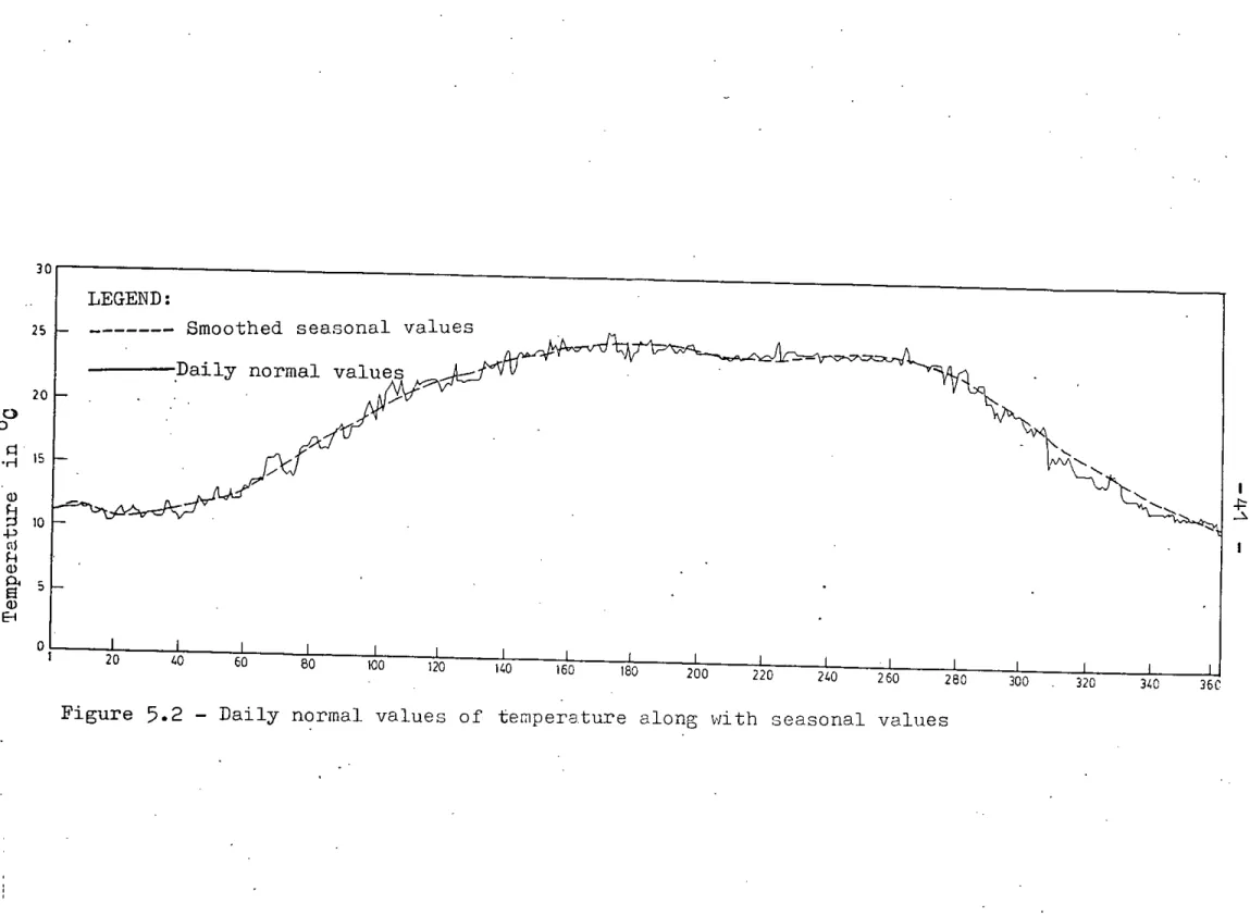
Daily normal values of temperature along with seasonal values

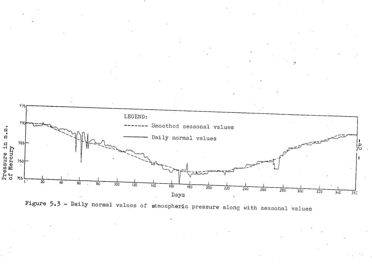
Daily normal values of .atmospheric pressure . alon~ with seasonal values

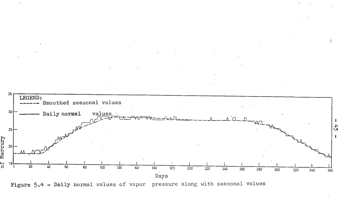
Daily normal values of vapor pressure along with seasonal values

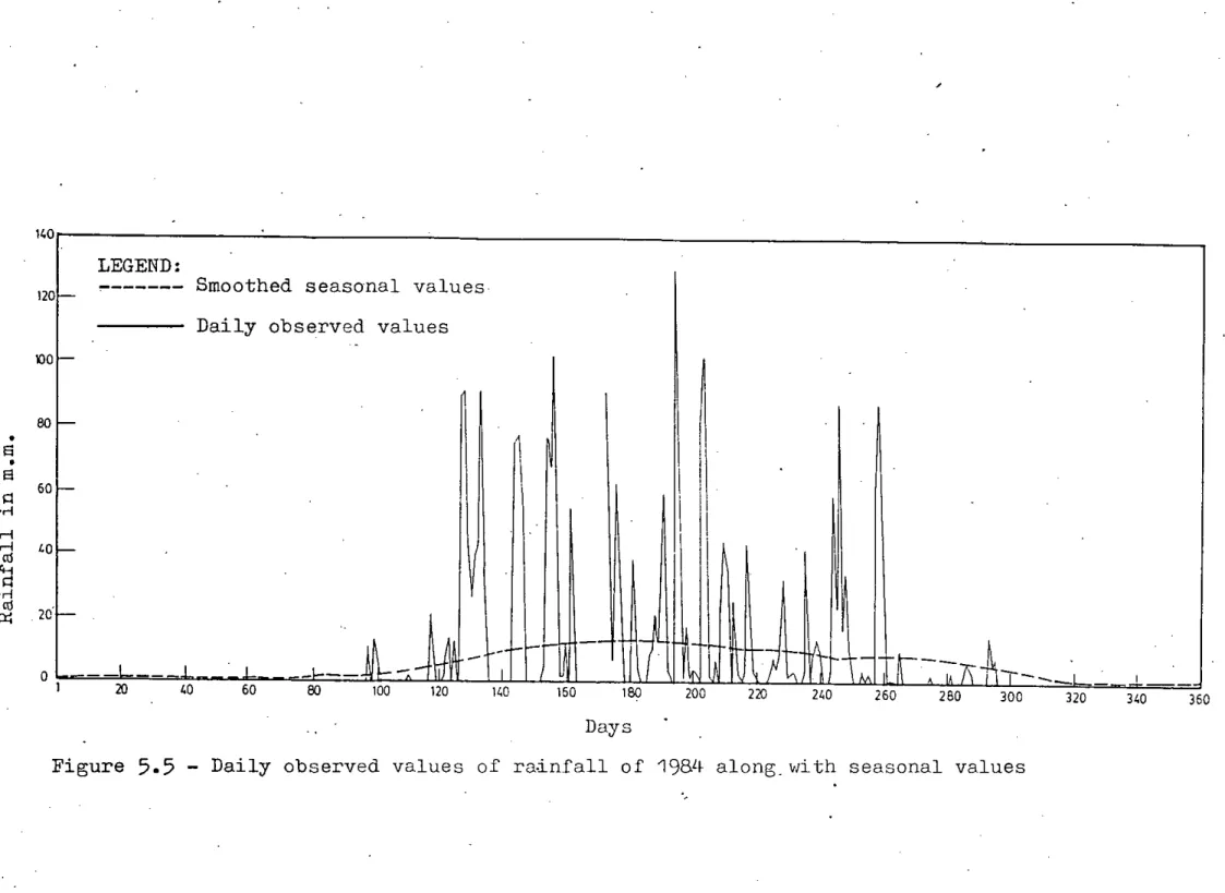
Daily observed values of rainfall of 1984 along with seasonal values

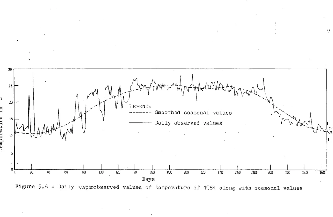
Daily observed values of temperature of 1984 along with seasonal values

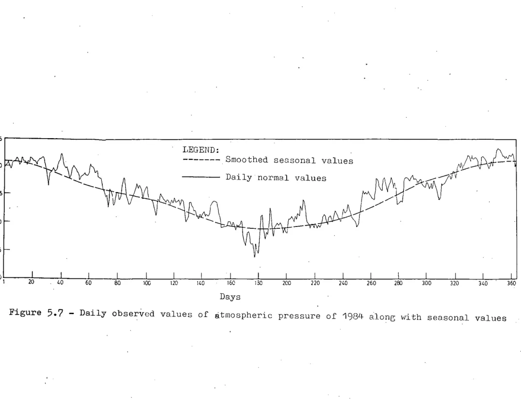
Daily observed values of atmospheric pressure of 1984 along "vith seasonal values

Daily observed values of vapor pressure of 1984 along with seasonal values

Daily observed values of rainfall of 1985 along with seasonal values

Daily observed values of temperature of 1985 along with seasonal values

Daily observed values of atmospheric pressure of 1985 along v~th seasonal values

49

50 13.

14.

15.

16.

Daily observed values of vapor pressure of .1985 along with seasonal values

Daily observed values of rainfall of 1986 along with seasonal values

Daily observed values of temperature of 1986 along with seasonal values

Daily observed values of atmospheric pressure of 1986 along with seasonal values

51 52 53 54

Figure 17.

18.

19.

20.

LIST OF FIGliRES(Contd.)

Daily observed values of Vapor pressure of 1986 along ':Iithseasonal values

Predicted and observed values of daily rainfall for the year 1984

Predicted and observed values of daily rainfall for the year 1985

Predicted and observed values of daily rainfall for the year 1986

x

Page

55

.56 57 58

INTRODUCTION

1.1 Background

i

Bangladesh lS mostly a deltaic plain which lS devastated by flood almost every year. While containing the flood by

structural measures is a colossal enterprise both technically and econom~cally, non-structural measures like flood forecasting may be adopted with due care to alleviate the sufferings of the people.

Generally, a flood forecasting scheme has tliObasic components, namely a rainfall-runoff moeel and a routing model. The rainfall-runoff model estimates the fraction of rainfall that finds its way direct~y into channels and the

routing model delineates a flood wave down a Ivatercourse from r,.

knovin values at an upstream point. On small catchments, the two basic component models together do not provide enough lead time for evacuation ane other emergency measures. So for floods in small.catchments, known as flash floods, a third component, a rainfall forecasting model has been adopted in some very recent forecasting schemes (Georgakakos 1986Y. ^Besides

flood forecasting, rainfall forecasting may be of immense help to farmers whose cropping strategies are mostly .influenced by the variability of rainfall experienced at the begi~~ng and

- 2 .,.

end of rainy season. In rainfed agriculture, many agricultural operations revolve around the probability of receiving given amount of rainfall.

Rainfall forecasting is not an easy task. The complexity and variability of meteorological factors have always thwarted human efforts to forecast rainfall reliably. The prime need of rainfall forecasting to be reliable and useful is accurate and well distributed observational data from an adequate representa-"

tive net 1;lOrk.But in Bangladesh data collection net \-lorkof the meteorological variables are sparse, so only point observations could be used for this particular study.

In literature, extensive usage of statistical and probabi- listic techniques for rainfall modelling can be found. But the only significant achievement in the development of causal model has been reported by Georg~~akos and Bras

(1984).

Georgak~~os and Bras

(1984)

have proposed a rainfall model based on cloud micro-physics principle. The input variables are hourly ground station data on temperature, humidity and atmospheric pressure. They have successfully applied their model to storms

at Boston (Massachussetts) and Tulsa ((Oaklahoma).

So far, no attempt has been made by any researcher in Bangladesh to statistically correlate atmospheric pressure, temperature,and vapor pressure measured at ground level with

,

rainfall. This has encouraged the author to take up the study.

In the present study, it is proposed that further.improvement to the model developed by Georgaka~os and Bras can be achieved by incorporating seasonal information in the causal model. The methodology and assumptions for the development of the proposed model will be followed as given in Nash and Barsi (1983). Nash and.Barsi (1983) developed a hybrid model for forecasting stream - flow. This model considers streamflow as a function of rainfall and it has two components, namel~ the seasonal model and the linear perturbation model. The seasonal model deals hith the determination of seasonal values by fittin

o

Fourier series. to the data of the variables. The linear perturbation model regresses the deviations or perturbations of the observations from the

-

corresponding seasonal values of the dependent variable on those~

of the independent variable •

In the present study, the proposed model for forecasting rainfall is a hybrid model. This model considers rainfall as a function of atmospheric pressure, air temperature, and vapor pressure measured at ground level. Following the methodology of Nash and Brasi (1983), it is intended that the seasonal values of all the variables will be achieved by fitting Fourier series to the daily normal values known as 'the seasonal model' and a linear regression model will be developed to,correlate the per- turbations of the meteorological variables with those of rainfall.

- 4 -

The principal component regression technique will be performed to transform the mutually correlated variables into mutually uncorrelated variables. For easy comprehension, the definition sketch of the seasonal values and perturbations of a time series is given in Fig.1.1.

deviation or perturbation

seasonal value obt~ined by fitting Fourier series

1.2 Objectives of the Study

The main objective of this research is to develop a hybrid model for forecasting rainfall. The model considers rainfall as a function of atmospheric pressure, temperature, and vapor pressure. The model has two components, namel~ the seasonal model and th~ linear perturbation model. The objectives of the study may be summarized as follows:

i. to develop a seasonal model to achieve seasonal values of all the variables.

-;,

ii. to develop a real-time rainfall forecasting model using observed meteorologic data which are found to have

significant contribution to precipitation generation.

iii. to evaluate the performance of the model uSlng different statistical tests such as t-statistic, F-statistic,

coefficient of determination~and coefficient o'f . efficiency.

'j

CHAPTER 2.

STOCHASTIC AND CAUSAL RAINFALL MODELS

Meteorologists and engineers have given serious attention to rainfall forecasting only in the last three decades. The primary emphasis has been to use statistic~procedures to model rainfall. The early works use pro.babilistictechmques linked to both space and time. The probabi~istic models suggested for rainfall prediction have evolved from the alternating renewal models (Green, 1964, Grace and Eagleson, 1966), to Poisson models (Duckstein et al, 1972), JVIarkovchains (Smith and Schreiber, 1973; Coe and Stern, 1982;.SrikanBmn and McMahon, 1982),discrete autoregressive moving average models (Chang et al., 1984) and to point process models (Kavvas and Del:eur, 1981; Smith and Karr, 1983, Rodriguez - Iturbe, 1986). Rodriguez- Iturbe (1986) and rtodriguez - Iturbe and Eagleson (1987) describe Poisson rectangular pulses model and Neymann-Scott rectangular pulses model. They have extended these models at different levels of temporal and spatial aggregation. Foufoula - Georgiou and Guttorp (1986) have pointed out the limitations of Neymann-Scott models.

Any effort to model rainfall at short intervals of time should envisage two aspects. The first aspect is to model the probab~lity of having either a dry period or a wet period. The difference between a wet period and a dry period may have a predefined threshold value of rainfall. The simplest model for this purpose is a Poisson model.

Poisson process is indepen~ant of time and does not contain any

seasonal variability. The other aspect is the amount of rain falling in a certain amount of time.

I

Ozturk (1981 )presented~a model for amounts of rainfall.

According to him, if rainfall is taken to be a Poisson process with mean intensity _\ , number of showers in time interval t is

\^..•..

e~

^~)and rainfall amounts of single shower is taken to be exponentially distributed wi~h mean ~ ' then the cumulative distribution function of amount of rainfall, X is given by

, OC

-8 '-

e-+-L.-

, . \<--:- ,

'Woolhiser and Roldan (1986) combined the two aspects of the rainfall model. They developed a stochastic daily rainfall model.

They used a first order Markov chain with transition probabilities

F\(n)- p(Xh=j\

^X

h _\=)

: 'j fJ1

1

'n

= \~

^{2J" •... J} "3 C!::>

\;J""=-u,.,

where state 0 signifies a dry d~T and state 1 a wet day and

P

1('h)

= ^{'1- P. oCYl)}

,~ \ \

If yet), the amount of rain~all that falls on day t, is assumed to be serially independant and independent of Xt_1, then it follows that the random variable Ut = Yt - T can be represented as a mixed exponential distribution with probability density function:

0<.

en)

pen)

o

-<

1).. :::; ex; •

o ::; 0<

(:n')

< \

,

'n = \, "2., .... -.> ::bcS

- 8 -

The mixed exponential distribution can be interpreted as the result of a random sample from two exponential distributions where the distribution with the smaller mean ~(n) is sampled with probability

,

I

mean

'ben)

^is

O«n) and the distribution with the larger sampled with probability ( 1 - C«n».

Woolhiser and Pegram (1979) have shown that the seasonal

five.p~rameters of markov chain and two can be described by the polar form of a variations in each of the

exponential distributions finite Fourier series:

where i = 1,2, ... , 5, jJ{(n) is the value of the ith

parameter on day n, n = 1,2, ... ,365, mi = maXlmum number of harmonics for the ith parameter, ~io=r mean of each parameter.

c ..

= amplitude, and jZl-.. = Phase angle. W oolhiser and Roldan

lJ - lJ

applied the above model to 16 stations in south Dakota and

obtained concise description of seasonal variation of parameters

•_". by using from 15 to 27 coefficients; but they also found spurious variability in parameters.

Several other investigators have proposed stochastic models describing both rainfall occurrence and its distribution in

amounts at a point in space (Jones et al., 1972, Smith and Schreiber, 1973, 1974; Todorovic and Woolhiser, 1975;Haan et al., 1976; and

Katz, 1977).

To predict rainfall at longer intervals of time, e.g., monthly or yearly, the interest is only in the quantity of rain; that falls at-a time step. SrikanBmnand McMahon (1982). applied to five Australian

rain gauge stations a first order Markov model; that preserved annual auto-correlation in the form

"'{L '

X t:.'= f:x ^l:-\ + (\- ^{5') Eo\::}

\J

.\ where Xt is stalrlardizedrainfall in year t,

S

is lag 1 auto-

correlation coefficient, and

E\

is white noise i~ fitted rainfall data have ne~ligible skewness. If there is signific2nt skewness with coefficient ~, the noise term should be subjecte~ to Wilson Hilferty (1931) transformation as follows

" )"1.-- ,

Yn "\, _-\)i '3c:;. ~

,

Srikanthan and McMahon suggested disaggregation procedure as

~ given by Valencia and Scha~~e (1973) to generate monthly rainfall forecasts from annual serles. However, they found that the simple method

of

fragments gave better results than the disaggregation scheme. Coe and stern (198?) describes a second order Markov chain which they fitted to rainfall data of Jordan, Niger, Botswana and Sri Lanka.

The above probabilistic models have been quite

successful in rainfall prediction, but yielded only limited success in rainfall forecasting because the rainfall• correlation structure is generally quickly decaying. Therefore, these sophisticated

models have little value in real-time forecasting. Nevertheless,

- 10 -

rainfall is non-linearly related to a series of meteorological variables, which in turn exhibit slowly decaying correlations and high cross-correlation. Their forecasting, using statistical

•

•

techniques, is then feasible. Georgakakos and Bras (1984) have proposed a rainfall model based on the conservation of condensed water equivalent mass in a cloud column characterized by the input variables of ground station data on temperature (Td),dew point temperature (To) and pressure (P~).'CloUd microphysics gives' expressions for the rainfall rate as a function of the input

variables, the model state, ,and the storm invariant parameters.' Pseudo adiabatic condensation gives the input rate in the cloud column. Temperature, Humidity and Pressure values are presently well predicted by statistical techniques like the model output statistics method of the Techniques Development Laboratory of the U.S. National \JeatherService (Glahn and Lowry, 1972, Lowry and Glahn, 1976).

In brief, the model equations of Georgakakos and Bras are

fp (xp• u

,

~p) = f(~) - h(~) x (1)

p where f(~) =~;o

- w

(Tt,

~

e

^{mov (2)}

s

~ = (Ps/RTs ₊ Pt~RTt)/2 ⁽³⁾

Wo = W (Td, P ) (4)

s 0

EA

(T - 223.15)3.5

Ws (T, P) ₌ 1 (5)

P 12

v =

E

^{1 r-}

_IC

^{(T -} T'

)l

₍₆₎

~p m s .--1.

P = (

s

+ 1 )

3.5

po

T ( 1

)T (8)

s

=

To - Td _+:1. ⁰ 223.15

T0 0.286

T'_S

=

^(pI)

(9)

pO•286

0

pI = 3 p +

1

^Pt (10)

4 s 4

The temperature Tm and the pressure Pt are found as the solutions of the system of algebric equations;

P 0.286

Tm ( _n_)

P'

t

^{L(T) W (T ,P')}

exp m s m

C

^m

T

^{m (11)}

- 12 -

<::-2- PL Pt

=

^{Pl +}

1 _+~ (Op (Tm - T's

))~

with

Pn 0.286

t

^{L(T)W (T p) ~,i}

Q^e

=

^{Ts (}

J?

^{s ) eXD . s0psTs s, ,s}

J

( 12)

L('r) = A - B (T - 273.15) (14)

The temperature Tt is found as the solution of the algebric equation,

The function h (~) In (equation 1) is given by

r

^{1 +}

^.2

^{N + Nv2 N3}

V 4 v

-zr

⁺ ₂₄v

" ^h(~)

-2

c

S ^,

^,\_L- N

e v

~ ~ (YNv) +

(iN )2 (J

^{N )3}

1 v v

4 + 24 N

1\ (16)

+ + v

4y4 +

-/5 e-J

N

Y5.J

v

I

~

"

I,,

Vp = 4 0(

E

4 vID

Bv (1-m) Nv= ---

4

( 18)

,r

,

\:

"

~

1 ₍ 1 1 1

=3 )' + .)""V + ..i2)

R(Ts + Tt) P

Z ln ( s

)

= Pt

c 2g

':rheobservation function h (x ..

!:!

,

~p) is given by

p p'

r _{4DAB es (Tw) e (Td)}

J'/3

D

= ~~ Zb ⁽ s

c Rv T_w To

es (T) = A1 (T - 223.15)3.5

(20)

(25)

(26)

, .

- 14 -

ln

p (_0_)

ps

(28)

The temperature Tw is the solution of the algebric equation,

T = T

w 0

The diffusivity of water vapouT in air varies with temperature T and pressure F according to

o 0

(30)

* (+)

o.

) is the scalar function to represent the

--)

T DAB ₌ A2 ( _T⁰

•

where

Function .l.^~ ( P

time derivative of the precipitation model

Function h (

P

state~

) is the scalar function that gives the

relationship between the precipitation rate observed and the hydrometeorolosical model states.

Xp represents precipitation model state.

u represents precipitation model input: T

0'

a represents vector of precipitation model storm-invariant-

-p

parameters (E^{1, 02,}

c

3, ^{°4, -) , ~ , m )}

and Zb are the top elevation and the bottom elevation of the Zt

i

r

_{Ps .and}^cloud

colunn

column respectively.

Ts are the pressure and temperature of the bottom cloud respectively.

,

r.

, Pt and Tt are the pressure and temperature at the top of cloud column respectively.

R is the gas constant.

C lS the specific heat at constant pressure.

p

P is the nominal pressure.

n

L(T) is the Latent heat of condensation.

Vi (Td, P ) is the saturation mixing ratio at temperature

s 0

T and pressure Po.

d

,es (Td) lS the saturation vapour pressure over a plane surface of Dure water.

.

^,

J?m is the vertically (inside the cloud) aver~ged density of moist air,

) is the ratio of the average diameter at cloud base to the average diameter at cloud top.

Z is the heiGht within the cloud measured from cloud bottom.

Z is the thickness of cloud column.

c

Wo is the initial mixing ratio of dry air.

Nash and Barsi (1983)dev~IBd a hybrid model for streamflow forecasting. The model has two components, namel~ the seasonal model and the linear perturbation model. They developed the model based on the following assumptions.

i. If. every input function, for each day of the year is equal to its expected value for that day, the output will also equal its expectation for that day.

- 16 -

ii. Perturbations x, or departures, from the daily expected values, in the inputs are linearly related to the

correspond~ng. perturbations y in the out-put.

Notationally,

where xi =.Ii - id; Yi = Qi - qd

o. and I, are the obse~ved outflow and observed input

"J.

^l.

(rainfall/upstream inflo\v) respectively.

qd and id are the seasonal mean discharge and seasonal mean input respectively.

The expected values or the seasorlal values have been

achieved by fitting Fourier series to the data. The deviations .or perturbations of the dependent variable from the seasonal

values are linearly regressed on those of the independent

variable. Their model yielded results with reasonable agreement.

In the present st~dy, the meteorological variables atmospheric pressure~temperature.and vapor pressure will be considered ~s the significant factors for producing rainfall as identified by

Georgakakos and Bras and the assumptions and techniques of

solution as described in Nash and Barsi (1983) will be applied.

c.

PROBLEM FORtWLATION AND ~lliTHODSOF SOLUTION

3.1 Introduction

The primary aim of this study is to develop a hybrid wodel for forecasting rainfall. 'rheproposed model compries two com- ponents, namely the seasonal model and the linear perturbation model. The model considers rainfall as a function of atmospheric pressure, temperature and vapor pressure. The seasonal modelling is done by fitting Fourier series to the daily normal values of all the variables. The linear perturbation model described in the sequel is a very simple model that yielded astonishing results

with streamflow forecasting (Nash and Barsi 1983). The t-statistic, F-statistic~coefficient cf determination, and coefficient of

efficiency used in this study are perhaps the most commonly under- stood performance indices among a myriad of statistical testing

, procedures.

3.2 The Seasonal Nodel

Following the assumptions as stated earlier'of Nash and Barsi (1983), it is proposed here that seasonal values of atmospheric pressure, temperature and vapor pressure are assumed to generate s~asonal values of rainfall

and the

deviations of individual events of atmospheric pressure, tem-.

perature, and vapor pressure from their seasonal values are

- 18 -

ii

I

I

,

I

pressure (ht), and temperature (Tt) equal the simple seas~nal mean valuesPt,

h

t and Tt for that time period, the corresponding rainfall would also agree with its seasonal mean value Rt•

Hence, it follows that

(Pt

,h

^t

,T

^t)-7Rt

for each time period t, "here the bar indicutes an average for that time step estimated over n years of observation which is taken as an estimate of the seasonal value for that time s~ep.

Intuitively, the population Pt, ht and Tt series are sillooth,I'

so the estimates obtained by simple time averaging are thej~ smoothed by harmonic analysis to yield more realistic estimates. Thus,

Fourier series of a few harmonics can be fitted separately to the

, ^\

mean values of eaC'ltime period of atmospheric pressure, temper2.ture, vapor pressure, and rainfall of the form (for daily basis):

~ [a.

^{m Cos}

(-::J.mn'K/~C.5)

+

b

^m

^~\n

^(';l.nm

k/'3=)J

^(3.1)

m=\ .

5(= (3.2)

"l..

-

-

_3cS 0.4-)

the basis of the proportion of total variance ( ¹ )65

O.5'(a~

+

and ~ is the total number of harmonics required to represent the seasonal values which is adopted in a particular case on

)*L(x _31')2

k b~) •

accounted for by the variance of pth barmonic

The nel'!values obtained by Fourier smoothing are designated as seasonal values of atmospheric pressure, temperature, vapor pressure,and rainfall.

3.3

The Linear Perturbation Model

It is postulated here that in any observed record, the series of departures of atQospheric pressure, temperatUre, vapor pressure, and rainfall from their respective seasonal values are linearly related by a simple linear regression relationship, as follows:

where the vector

Q

represents regression coefficients ~~d ed lS

error term. It is reasonable to expect significant cross- .correlations among pressure, temperature, and vapor pressure.

/

In performing multivariate analysis, many methods are found in literature such as principal component regression, ridge regression, latent root regression, cannonical correlation, factor analysis etc. In this particular study, the principal component regression technique has been adopted. Hence the salient features of this technique is described below.

20

The objective of principal component analysis is to transform the original correlated variables into uncorrelated or orthogonal components. These components are linear functions of the original variables. Such a transformation can be 'dritten 0.3

w

⁼ Z A 0.6)

where Z is an n x p "raris"lce .-;ovariancematd)cor correlation

\

matrix of n observations on p variables.

W is an n x p matrix of n values for each of p components.

A is

a

p x p orthogonal matrix of coefficients defining the linear transformation.

In ,:JerforminSthe multiple r.egression on principal components, the independent variables are standardized in order to avoid the vroblem of noncomrnensurate units of the variables lli"ldthe dependent

variables centered so that

I

1 i

\

(3.7)

when Ztj =

-

xt. - x .

.l .l

S.J

t = 1,2, ,n, j = 1,2, p

x is the mean of the J.thvariable

j

Sj is the standard deviation of the jth variable.

Xtj stands for ~Pt, A-ht or .ATt.

It should be mentioned here that the centering of the

dependent variable is not necessary. It eliminates the need for an intereept and simplifies notation.

The correlation matrix is given by: S

=

_{(n-1 )}

Characteristic roots (sometimes called latent roots or elgen

0.8)

valUes) of this correlation matrix are the p solution

•••••• of the determinantal equation p

Here p lS the number of variables

1 '

•

Associated with each characteristic root; j; is a characteristic vector,

The solutions ~j = (a1j, a2j ••••• apj), chosen from the

\

set of equations

a., which satisties the homogeneous -J

(~ - ~j

! )

~j =

9

^0.10)

"

"

infinity of proportional solutions that the normalized solutions such that a.T,

<.I

components ~IS e..rethen computed as

exist for each j, are a. = 1. The principal

J

the new Wj column wit~ elements Wjt,

~j = a1j Z1 + a2j Then sum of squares of

Z2 + •••• ~•.•• , + a . Z pJ P

t = 1,2 ••.. , n is j' Also it can be shown th~t Hence ~ vectors are orthogonal to each'other.

The ~j corresponding to the largest " value lS called

u

the principal component and it explains or accounts for, the largest proportion of the variation in the standardized data set. Further, W.' s explain smaller and smaller proportions

-J

until all the variation is explained. That is,

The jth principal component accounts for 100 CX./Trace S

. J -

percent .of the total system variance.

The correlation between the ith standardized variable and the jth principal component is given as

Cor (zi'Wj) = <.Aj .aij 0.12)

- 22-

Typically one does not use all the ~j'Sbut follows Borne sort of selection procedure. Some psychologists use the rule that only eigen values greater than 1 are of interest. D.F.

Morrison (Draper and Smith, 1981) suggests that "••••components might be computed until some arbitrarily large proportion

(perhaps 75 percent or more) of the variance has been explained", that is, the set of largest k contributors \ihich first achieve

i,C).,j!-o

^/0.75 has to be selected. Some such rule automatically provides with a set of \<W's and the original "?~s are then

transformed into this set of

k new ~predictor vccriables.

The regression model, then, may be described as

p

'IS

=?

t3j W

e,-

-+

e

t:

t ,.f=I ;)

In matrix form, equation

(3.11)

turns out to be R=\I'B+E

where, R lS a vector, ~1' ~, ••.• , 15~T

B is the vector of regression coefficients,

I'

E is the error vector,

I!1'

^{e2, ••••• e. -, T}n)ⁱ

T

~ l'

B

^{2, ••.•}

BPl

C3 .14)

If b be the sample estimate of the vector ~using least square criteria, then it can be shown with the help of matrix algebra that the normal equations corresponding to equation

(3.11)

takes

the form:

[!i? ~"] ~ =

'!iT ~ C3.1 5)

where ~T is the transpose of the matrix W. The solution matrix

\.

for sample estimates of parameters becomes:

-1

_b =

L

^{w.Ty ] X{TR} _(3.16)

After estimating, the regression coefficients, the result of aregression on principal components can be transformed to an

equation in terms of the original variables. In doing so, equation (3.13) becomes

,.

_P

b. {~ 0."['X6:-~JJ

ARt

=

^{.oR +} _'Z:

J ^{\<= \} "'J, ^SI<.

j

=

¹

I'

',.

^{or .bRt}

=

^{.a.R+ b1A ht +}, ^b2 AT t ₊ b3~Pt (].17 ) 3.4 Inferences on Regression Coefficients

To make inferences concerning B, the variance of b must be known. The variance-covariance matrix of

3

^{lS given as:}

Cov(:\2)

, -1

6.2 (".'T,,)

= ./ v

-

^-

The variance of bi is and is therefore ()2

The covariance of hi

(~T~)-1.

equal to the covariance of bi with itself

, , h f' (,/T,/)-1 .

tlmes the It" diagonal element o~ ~ ~' IF Vlithbj is 62 time~ the (i,j)th element of

It can be sho'.m that

--' '-

1 '?,

n-1

o

o

and

~r

bj

= ;Vlg /

^(n-1)'Aj

=

9--j^TZT

J./

^(n-i)'7\j

The derivations are given in Appendix-I.

From the above results Cov (bi, bj) = 0

=

^var

it-is apparent that for i # ^j

(b.) = <sV

/C'h-D"Aj

J

(3.21 )

where Clis the standard error of the regression equation. Thus Q

i

is independent' of b j for i # j. The independence of the

.E

^Is

lS a result of the orthogonality of the principal components.

- 24 -

If the model lS correct, then the quantity bj/sbj is distributed as a t distribution with n-p degrees of freedom where S~b' is an estimate for Var(b .). To test the hypothesis

J . J

that HO:Bj = 0.0 against Ha:Bj

#

0.0, the test statistic for the statistical significance of B. is

J b.

t = J (3.22)

Sbj

Equation 0.20) can be \vritten as t = g..~'z.TRrJ!['-\)9\~6 0.23) Here HO lS rej ected if \t

,;>

^{t1..9Y2 n-p} which means that the jth independent variable is contributing signific:mtl:7

to explc,in the variation in the depen~~ent vCTiable. Alter:l2.tively, if the null hypothesis is accepted, then the corresponding

independent variable is usually deleted from the model. There is no reason to believe before the regression is performed that

this test statistic will be non significant for small values of

~j .

^Therefore, the regression should be performed on all of the components and then the components that prove to be non- significant can be eliminated.

A test of the hypothesis that the entire regression equation is not explainlng a significant amount of the variation of the dependent variable, the null hypothesis will be HO:B1 = B2 •••••

Bp

=

0.0 versus Ha: at least one of these B's is not zero. Here use is made of the fact that the ratio of the mean square due to

regression to the residual mean square has an F distribution with P-1 and n-p degrees of freedom. The F statistic in matrix form

may be given as:

F =

C ~T~TB - n

R

2)/CP-1)

C~T~ _ £T~:g)/Cn_p) ^0.24)

r I

Rejection region : F~ F1_~,

/ ~ P-1, n-p.

3.5 Coefficient of Determination and the ANOVA Table For assessing the adequacy of the model, one approach

that does not involve an;}'assumption," is to determine ho\'!much of the variability in the cepen~ent variable is explained by the reGression. 'l'hevariability in the depencent vClriaele R is quantified as a sum of squares. The error sum of squares

SSE =

2:

^{CRt -}

R

t)2 measures how much variability in the Rt,s is not e;~lained by the regression relationship. If SSE is quite small, all the observed pairs lie near the least

square line, while if it is large, then there is much 'residual variability' even after taking into account the possibility of a linear relationship.

The total amount of variability in the Rts can be measured

, - 2

by computing SST =

L:

^CRt-H) which is the total sum of squares of the, Rt, s about their mean. Hence,the coefficient of multiple regression R2, indicating the proportion of variation in Rt,s explained by linear regression is defined as:

=

1 -

"

= (SST - SSE)

SST

SSE SST

r'_"

- 26 -

The table given below, called the ANOVA (analysis of variance) table is quite helpful in calculating all the above terms and for other analyses using matrix notation.

ANO\TATABLE Source

~lean

Regression Resid.ual Total

Degrees of Sum of

freedom squa.res

.'1 n R^-2

P-1 bT\yTR -2

- n R

- --

n-P RTR _ bT'IiTR

- - -

n RTR

f, .

I I

r

- -

Using the ANOVA table, S3'r, SSE and R2 assume the following forms:

SSJ: RTR -2

= - ^- -

^nR

SSE

= - -

^RJ:R

-

^bTWJ:R

^- --

^{(-~6'5.c:. -'}

R2

=

^(~J:.lFB

- rill

^2)/ (~T!,

- ^rill

²⁾

Another important statistic, Var(e) or (52 is represented by its sample estimate s2 as: 2

S =

which lS also known as residual mean square.

3.6 Evaluation of the Model Performance

In order to evaluate the performance of the proposed hybrid model, the predicted values of rainfall will be compared with tpe observed values. The coefficient of efficiency' which is extensively used in evaluating the adequacy of the model will

• also be determined. The coefficient of efficiency is defined as:

- 2 ^A. 2

Z (Rt - R) - 2:"(Rt - Rt)

2- (Rt - R )2

(3.28)

where Rt is the t-th observed value of rainfalL

"-

Rt is the t-th estimated value of the rainfall

R

is the mean of the observed rainfall values •.

"

If all Rt

=

Rt, then Ef

=

1. For any real situation, Ef

<

1. It is possible for Ef to become negative; a negative efficiency infers that the model's predictec value is worse

than simply using the observed mean. Large events are 'ieit;hted in equation (3.28 ); thus an efficiency can be biased i'fhena large range of events are evaluated.

3.7

Develoument Procedure

The step by step procedure for the development of the proposed model is enumersted and described belo,l:

a. to calculate the mean values of all the variables;

b. to smooth the daily mean values by fitting Fourier series of a few harmonics;

c. to subtract the seasonal mean value (in cycle of 365 for daily) from each of the observed value over the full period of calib.ration in order to obtain the perturbations of individual events;

d. to standanlize the perturbations of the independent variables and center the dependent variable, that is,

andR =

z =

is,

- 28 -

where Ztj = and

I I

AX.

^{and S.} are the mean and standard deviation of the

J J

perturbations of the jth variable respectively.

~Rt is the mean of the perturbation of rainfall;

e. to compute the correlation matrix of the input variables (independent variables)

s =

f. to compute the eigen values the corre~a.tion matrix;

and elgen vectorSJf of

g. to calculate the values of the principal components ~;

h. to estima~e the values of b and then to compute the estimated perturbation of ~ainfall;

l. the estimated value of rainfall can t;lenbe computed by adding the seasonal mean rainfall Rt to the estimated

A

perturbation series LlRt in a cyclic manner (i.e., 365 values of Rt repeating for each year of the record on daily basis)

II

DATA COLLECTION, DATA PROCESSING AND CCr'IPUTER PROGRA1'If''lING .

4.1 Sources of Data

The rainfall forecasting model in its development and testing requires the following data:

l. daily mean n.infall ii. daily mean tempers.ture

iii. daily mean vapor pressure and iv. daily mean atmospheric pressure.

For proper development, spatial distribution of these variables over a catchment is preferable, but in B2~6ladesh data collection net work of all these meteorological variables are sparse, so only point observations could be used for this particular study. The point observations of rainfall, pressure, temperature and vapor pressure of a rain gauge of Dh~~a City have been used.

4.2 Data Collection and Processing

Daily mean rainfall, in m.m., daily mean temperature in 0C, daily mean at~ospheric pressure in mbar,and daily mean humidity for the period 1984 to 1986 recorded at a meteorological. station have been collected from Dhaka Meteorological Office. Daily

normal values of all the variables obtained from observed data from 1951 to 1980 have also been collected from the same office.

r

- 30 -

Daily mean humidity and daily normal humidity have been converted into corresponding vapor pressure in m.m. of Mercury using Regnault's Table. All the data have, then, been stored in the mainfra~e of the BUET Computer for further processing and analyses.

4.3

Computer Programming

In order to get daily normal values of all the variables, a computer program in FORTRAN IV language has been developed by the author and it has been run in the mainframe of the Computer Centre of Dhaka Meteorological Office.

For regre0sion analysis, the software 'SPSS' (Statistical Package for Social Science) available in the mainframe of BUET Computer Centre has been used. 'rhis package is an integrated

system of computer programs developed by SFSS Inc., Chicago, U.3.A.', for a wide ranGe of statistical analysis. Also, it provides the

user with a comprehensive set of procedures for data tra~sfamation and file manipulation. The package has been updated and recast several times •.The version of SPSS that has been installed in BUET main frame was first released in

1975.

Besides SPSS, the author has developed computer programs in FORTRAl{ IV language for fitting Fourier series to the daily normal values of all the variables, computing eigen values and eigen vectors, determining principal components and coefficient of efficiency of the model.

MODEL SOLUTION AND RESULTS

5.1 Introduction

The rainfall model described earlier has been developed and tested with daily values of rainfall as a dependent variable and atmospheric pressure, ieoperature, and vapor' pressure as independent variables recorded at a single rain gauge station of Dhaka City. As stated earlier, the model has two components, namely the sec.sonal model and the linear per- turbation motier. Follo\ving the development procedure as d.escri- bed e~rlier, the steps of analyses will be followed in detail and pertinent comments will be made.

"

5.2 DeveloDment of the Seasonal Model

The seasonal modelling was done by fitting Fourier se:':'les to the daily normal values of all the variables. In doing so, The Fourier coefficients a and b and the perc.entage variance

m m

accounted for by each harmonic cm were calculated using equations (3.1 ) to (3.4 ). The number of harmonics for each series was selected from variance analysis to be 5. The Fourier coefficients used for smoothing and variance explained by each harmonic are given in Table 5.1 ^through 5.4 for rainfall, pressure, temperature and vapor pressure respectively.

-'32 -

, Table

5.1:

Fourier coefficients and variance explained by each harmonic for rainfall data from 1951 to 1980

Number of Fourier Coefficients Variance accounted by harmonics

am bm the mth he.rmonic

1 6.17 1.84 20.76

2 0.76 0.23 0.32

3 - 0.26 0.83 0.38

Lj. 0.17 - 0.14 0.03

5 0.33 - 0.11 0.06

R~

=

~+

z' r

^{m cos (2/\rnk/365}

⁾⁺

^b_ill sin (2" ITLV365B

'0\." I

K = 1,2, 365

Table, 5.2: Fourier coefficients and variB.nce explained by each harmonic for 3.-::Josphericpressure data from 1951 to 1980

" Number of Fourier Coefficients Variance accounted by

harmonics

am bm the mth harmonic

1 - 7.74 0.28 17.33

2 0.36 0.72 0.18

3 0.33 0.19 0.042

4 0.10 0.38 0.043

5 0.08 0.05 0.0023

P1K = PI< +

~ Eln

_m'=l c.oscz-nm\<)_~c:s

-+

'bm

~,n (~"ml</:;c:.s21

Table 5.3: Fourier coefficients and variance explained by each harmonic for temperature data from 1951 to 1980

Number of Fourier Coefficients Variance'accounted by harmonics

a b the mth harmonic

m m

1 - 4.73 - 0.31 11.22

2 - 2.36 - 0.68 3.02

3 - 0.36 - 0.27 0.10

4 0.22 - 0.07 0.0268

5 0.07 0.04 0.0033

\3. .

T1( = TI<+ ~ [. a.m cos(~l\rn"'/;;cs)-+ bmS<illl("1.l1rnkhc!»]

Table 5.4: Fourier coefficients and vari~nce explained by each harmonic for vapor pressure data from 1951 to 1980 Number of Fourier Coefficients Variance accounted by h'armonics

a b the mth harmonic

m m

" '1 - 6.85 -2.37 ^26.26

2 - 1.42 - 0.97 1.4816

3 0.08 0.28 0.0433

4 0.30 0.007 0.0475

5 - 0.15 0.0029 0.0118

h

^k

= ^h

^-+

i-::,. [

^{<AmCo 'S} (~nm\o</~c:.s)-\-b

m

^S\Yl

(~nm\</:;c.s51

- 34 -

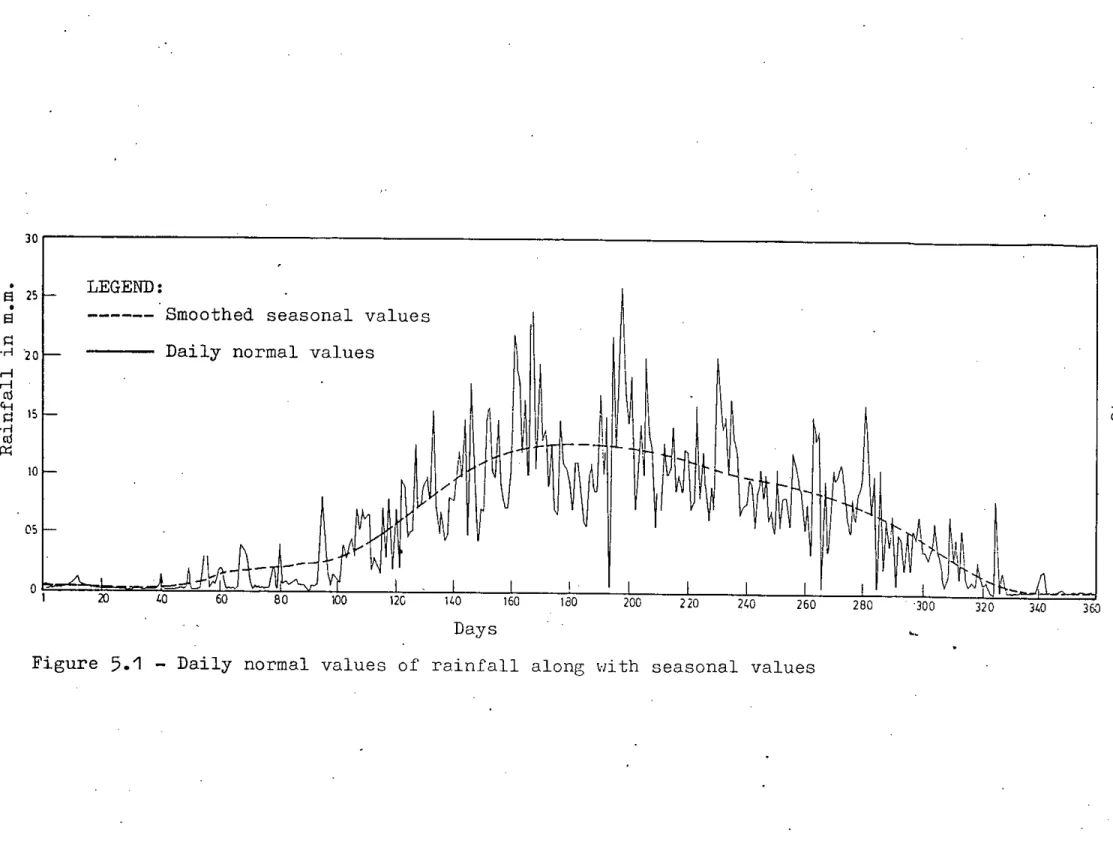
The smoothed data series of each of the variables ~hus obtained has been termed as seasonal values. A plot of the smoothed data series of each variable constructed from five harmonics is given in Figures 5.1 through 5.4 along with the daily normal values. These seasonal values were then subtracted from the daily values of all the variables from 1984 to 1986 to get the deviations or perturbations series. The perturbation series of each of the variables thus obtained were then applied to develop the linear perturbation model. The plots of the

observed values of each of the variables from 1984 to 1986 along 'dith seasonal values are glven in Figures 5.5 ^through 5.16. It is clearly evident that all the meteorological variables have high seasonal characteristics.

5.3

Development and Testing of the Linear Perturbation Model

Follo\'!ingthe development procedure as described in chapter 3, the individual v2,riables \Vere standardi zed using equation ( 3.7 ) and the 3 x 3 correlation matrix of the standardized variables was determined using equation

(3.8 )

arid is given in Table

5.5.

Table

5.5:

Correlation Matrix of the Standardized Variabl-es

ht Tt Pt

ht 1.00 0.61 0.22

Tt ^{0.61 1.00 - 0.14}

I Pt -0.22 -0.14 1.00

The eigen values and eigen vectors from the correlation matrix were then computed using equations ( 3.9 ) to (3.'10 ).

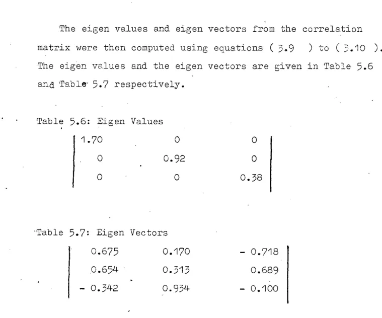
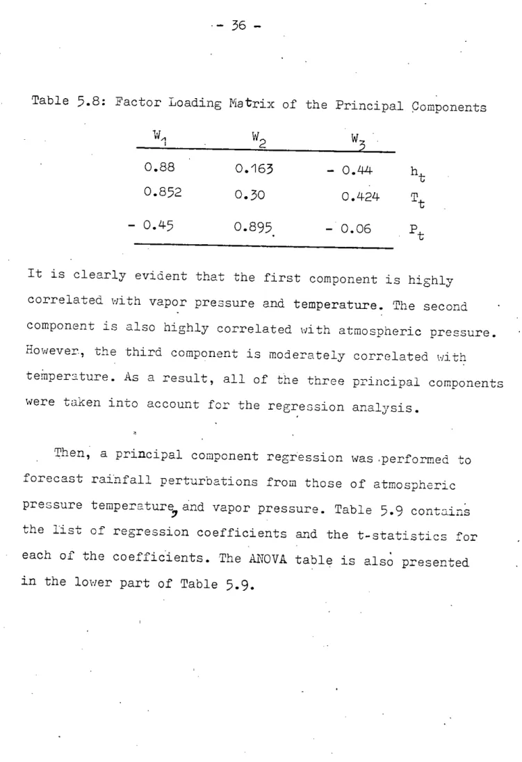
The eigen values and the eigen vectors are given in Table 5.6 and 'TabI.e' 5.7 respectively.

Table 5.6: Eigen Values

:~ 1.70

o o

o

0.92

o

o o

0.38

'Table 5.7: Eigen Vectors 0.675

0.654 - 0.342

0.170 0.313 0.934

- 0.718 0.689 - 0.100

It is, clear that in this formulation the first principal component accounts for 56.67% of the system 'variance' while the second and the third components account for 30.67% and 12.66% respectively.

The principal components and their correlation matrix were then determined using equations (3.11 ) and (3.12 ) respec- tively.The correlation matrix or the factor loading matrix is given,in Table.

5.8.

<-

36 -

Table 5.8: Factor Loading Matrix of the Principal (Jomponents

";11 W2 W3

0.88 0.163 0.44- ht

0.852 0.30 0.424 Tt

- 0.45 0.895 - 0.06 Pt

It is clearly evident that the first component is highly correlated with vapor pressure and temperature. The second component is also highly correlated \<Iith atmospheric pressure.

However, the third component is moderately correlated \'!ith

temper2ture. As a result, all of the three principal components were taken into account for the regression analysis.

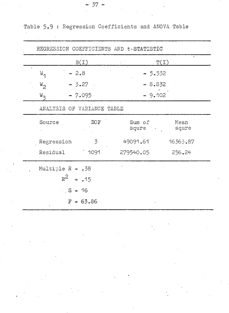
Then, a principal component regression was .performed to foreoast rainfall perturbations from those of atmospheric pressure temperatur~and vapor pressure. Table

5.9

contains the list of regression coefficients and the t-statistics for each of the coefficients • The AL'IOVA table is also presented in the lower part of Table

5.9.

Table

5.9

Regression Coefficients and ANOVA Table

REGR~S3lON COE~FlClENTS AND t-STATlSTlC

'.

^?'!

B(l)

\11 - 2.8

1;/2 - 3.27

\v - 7.095

3

ANALYSIS OF VARIANCE TABLE

T(l)

- 5.532 - 8.832 - 9.102

Source IlOF Sum of

squre

~lean squre

,_,.

Regression 3 Residual 1091 ['lulti;leR

=

^.38

R2

=

^.15

S

=

¹⁶

F

=

^63.86

49091.61 279540.05

16363.87 256.24

•

••

- 38 -

From the table it is revealed that all the principal

components are significant at 5"/0 level of significance (sig.^T= \":Jl(;;).

As given by the table, R2 is 0.15 in this case which means that the linear perturbation model has explained 15% of the total variation of the dependent variable. A further test of model utility may be done by F-test. The F value of 63.86 reported in this table is greater than the corresponding

critice.l vE,lue F1 c, 1 n (at eX = 0.05) of ~!-,c~• Clearly

- /' l p- ^l -p

the alternate hypothesis becomes accepted. The obtained regression equation has been expressed in terms of the original variables using equ8,tion (3.17 ) and takes the follOI'Jingforo:

5.4 'TheHybrid Nadel and its Performance

The seasonal values of rainfall obtained by the seasonal model were then added to the estimated perturbations of rainfall to obtain the total predicted values of rainfall. The hybrid model can be expressed in the following form

•Rt = Rt + 4.17 + 0.98 D ht - 4.47 6Tt - 0.52.dPt where

A

Rt is the t-th predicted valuest rainfall

R

t is the t-th seasonal value of rainfall'

~J:itis the t'th deviation of vapor pressure from seasonal value

DT is the t-th deviation of temperature from seasonal value t

6Pt is the tth deviation'of atmospheric pressure.

In order'to evaluate the performance of the model, the

coefficient of efficiency was determined as 0.23 using eouation

( j. 28 ) .Also the predicted values of rainfall for the y.ear1984 to 1986 are. compared with the observed values in Figure 5.17 to

5.19. It is evident that the model predicts moderate amount of rainfall reasonably well but poor agreement has been found between the predicted and observed values in case of high and low values of rainfall. This deficiency may be due to use ~f daily time step for the development of the model.

.,' 10-1; 4-.

30

S• 25

S• r:::

.rl "20 .--I .--I oj 'Hr::: 15

.rl

oj

po<

10

05

01

LEGEND:

--- Smoothed seasonal values Daily normal values

20

1\

Days

1801-

~II

1

_I 200

~

360 I

.J""

o

Figure 5.1 - Daily normal values of rainfall along 1"/ith seasonal values

30

LEGEND:

25

---

^Smoothed seasonal values

20

0°

q .rl 15

OJ

~ 10

+>

oj

~OJ

0.-S '

Eo<OJ

---D.ailynormal

-..y.

I .j:o

-"

01

20 40 60 80 100 120 140 160 180 200 220 240 260 280 300 320 340 36C

Figure

5.2 -

Daily normal values of temperature along with seasonal values

.-. .;o{ ,

.'

775

LEGEND:

I .p II\)

,<.

-^,.:\.

-.l3LO

-.l

320

-~

-

180 200

Daily normal values

Smoothed seasonal values

---

Days

Figure 5.3 - Daily normal values of atmospheric pressure along with seasonal values

s•

s

s:l .rl

t:

Q) ~

~ ~ ⁷⁵⁰

CJl Q)

CJl;:;:

Q)

H'H

7551 .

60

P-<o

<u LO

,

I

&

360 ...A.-_...<L.O - .1J----v:lfl

---

160 lea

==..='.b'=.=\ __

1,0

Daily normal

LEGEND:

--- Smoothed seasonal values

..J.1l.

151 30

25

• 35

s•

S

•..-l1'1

Ql

H;:l Ul Ul

~ ~ 20

H H;:l Ql

0:0:

P-

roCH

:>0

D~s

Figure 5.4 - Daily normal ~alues of vapor pressure along with seasonal values

" ^{-~ J;, ,}

,

140

j;

340 360 320

280 300 260

220 240 180 200

150 120 140

80 100

o 60

LEGEND:

~--- Smoothed seasonal values

)

Daily observed values

)

I

\

I

I I I

- -- _--

^{- I}

^--

, _... ... --

.~

_". ^{... ... -- -}

120

1:)0

80 S•

S•

~ ⁶⁰ .rl rlrl LO

ro

,rl~ p:;ro 20

0

D~s

Figure

5.5 -

Daily observed values of ra~nfall of 198L~along. with seasonal values

"

30

25

oo 20

>:l .rl

OJ 15

itl

~

H 10

OJ

0-S

OJ

E-<

5

01 20

jJtiY~\r/rV\~\~d\)

~EGEND:

Smoothed seasonal values Daily observed values

~~~

Days

Figure 5.6 - Daily vaparobserved values of temperClture of 198Lf along with seasonal values

~- :(. p

775

I

~

())

I

Smoothed seasonal values

LEGEND:

,v/VJ(\ ^VG,,~

^{Daily normal valuos}

iJX~~":\~

770

765

~760

()

I •.•

, eu 755

,;Z

,

I'Ho

75°1

Days

Figure

5.7 -

Daily observed values of atmospheric pressure of 198^Lf alone; with seasonal values

! '{

.0

I

.p-

-.,J I

3.0 360 300 320

280

-l260

Daily observed values Smoothed seasonal values

1.0

WIt!:W~/~L

20 I=l 30

•.-1

. Q) l»

H H.

g g

^2S

(JJH

Q) Q)

H:8 P<'H 20 H 0::s o •

P<El al • IS

:> El I

Figure 5.8 - Daily observed values of vapor pressure of 1984 along with seasonal values

.'