Assignment for Honours Part-III, Examination/2020

Assignment for Honours Part-III, Examination/2020

by Md. Atiqur Rahman

September 13, 2021

Chapter-2: Introduction

Simple interest rate

For the interest rate r the value V(T) at timeT of holding P units of currency starting at time t = 0 isV(T) = (1 +rT)P, where T is expressed in years.

Compound interest rate

For the interest rate r the value V(T) at timeT of holding P units of currency starting at time t = 0 isV(T) = (1 +_m^r )^mTP, wheremis the number interest payments made per annum.

Continuous compounding

For a constant interest rate r the time value of money under continuous compounding is given by V(T) =e^rTP.

Introduction

Return

Let us denote the asset price at timet by S(t). The meaningful quantity for the change of an asset price is its relative change ^∆S_S , which is called the return, where ∆S =S(t+δt)−S(t). In other words,

Return = change in value over a period of time initial investment

.

In the limit δt →0, its becomes ^dS_S .

Introduction

Simple Model for Stock Price dS

S =µdt+σdW

Deterministic part: This can be modeled by ^dS_S =µdt. Here, µis a measure of the growth rate of the asset. We may thinkµ is a constant during the life of an option.

Random part: The second part is a random change in response to external effects,such as unexpected news. It is modeled by a Brownian motion σdW, theσ is the order of fluctuations or the variance of the return and is called the volatility. The quantity σdW is sampled from a normal

distribution.

In other words σdW describes the stochastic change in the share price, where dW stands fordW =W(t+δt)−W(t) asδt →0,W(t) is a Wiener process, σ is the volatility.

The Brownian Motion (Wiener Precess)

A time dependent function W(t),t ∈R is said to be a Brownian motion if (a) For all t,W(t) is a random variable, i.e.

W(0) = 0.

(b) W(t) has continuous path, i.e. W(t) is continuous int.

(c)W(t) has independent increments. For anyu>0,v >0 the increments W(t+u)−W(t) and W(t+v)−W(t) are independent.

(d) For all σ >0, the incrementsW(t+σ)−W(t) is normaly distributed with mean zero and variance σ, i.e.

W(t+σ)−W(t)∼N(0, σ).

Normal Distribution

The probability density function for a random variable W(t) has a nor- mal distribution with mean µand variance σ², then the probability density function is

pW(t) = 1

√2πσ²exp

−(t−µ)² 2σ²

,−∞<t <∞.

The probability density function for a random variableW(z) has a standard normal distribution with mean 0 and variance 1, i.e., W(z)∼N(0,1) then the probability density function is

pW(z) = 1 2πexp

−z² 2

.

Properties

Show that

(i) E[W] = 0;

(ii) E[W²] =t;

(iii) E[∆W] = 0;

(iv) E[(∆W)²] = ∆t;

(v) ∆W =X(∆t)^(1/2),whereX ∼N(0,1)

Properties

(i) E[W(t)] =Rb

a tW(t)dt, for a≤W(t)≤b.

= Z _∞

−∞

√t

2πσe^−t

2

2σdt,putz = t² 2σ

=

√σ

√2π Z _∞

−∞

e^−zdz = 0.

(ii)E[W(t)²] =R_∞

−∞

t²

√2πσe^−t

2

2σdtputz = √^t σ.

=> σ

√2π Z _∞

−∞

z²e^−z

2

2dz= σ

√2π Z _∞

−∞

zd(e^−z

2 2)

= σ

√2π Z _∞

−∞

e^−z

2

2dz = σ

√2π

√2π =σ.

Question

1. Show that the return ^∆S_S is normally distributed with mean µ∆t and variance σ²∆t.

2. Show that ∆S ∼N(µS∆t, σ²S²∆t).

3. Show that lnS(t) is a normal distribution with mean lnS₀+ (µ−^σ₂²)t and varianceσ²t.

Answer

1. We have ^∆S_S =µ∆t+σ∆W =µ∆t+σ(W(t+ ∆t)−W(t)).

But µ∆t+σ∆W ∼N(0,∆t) =>∆W =X√

∆t, whereX ∼N(0,1).

Therefore, ^∆S_S =µ∆t+σX√

∆t,X ∼N(0,1)

=>E(^∆S_S ) =µ∆t+σ√

∆tE(X) =µ∆t+σ√

∆t·0 =µ∆t. Hence, mean=µ∆t Again,V(^∆S_S ) =σ²∆tV(X) =σ²∆t·1.

Hence, variance=σ²∆t

2. In similar fashion, we can prove question (2).

3. Solution of question (3)?

How to calculate small changes in a function that is dependent on the values determined by stochastic differential equation ?

Letf(S) be the desired smooth function ofS; sincef is sufficiently smooth we know that small changes in the asset’s price, dS, result in small changes to the function f. Recall that we approximated df with a Taylor series expansion, resulting in

df = df

dSdS+1 2

d^vf

dS²dS²+...; butdS²= (µSdt+σSdW)²

=>df = df

dS(µSdt+σSdW) +1 2

d²f

dS²(µSdt+σSdW)²+...

Assumption: As dt → 0,dW = σ(√

dt) => dW/vdt = 1 anddWdt = o(dt) =>dWdt = 0.

Implies that dS²→σ²S²dt as dt →0.

How to calculate small changes in a function that is dependent on the values determined by stochastic differential equation ?

df = df

dS(µSdt+σSdW) +1 2

d²f

dS²(σSdW)².

= df

dS(µSdt+σSdW) +1 2

d²f

dS²(σ²S²dt).

= (µSdf dS +1

2σ²S²d²f

dS²)dt +σSdf dSdW.

Itˆ o ’s Lemma

Statement: For any function f(S,t) of two variables W and t where S satisfies Stochastic Differential Equation (SDE)dS =µdt+σdW for some constants µ and σ, dW(t) is a Brownian motion (Wiener Process), then the general form of Itˆo’s Lemma is

df = (df

dt +µSdf dS +1

2σ²S²d²f

dS²)dt+σSdf dSdW.

Now consider f to be a function of both S and t. So long as we are aware of partial derivatives, we can once again expand our function (now f(S +dS,t+dt)) using a Taylor series approximation about (S,t) to get:

df = df

dSdS+df

dtdt+ 1 2(d²f

dS²dS²+d²f

dt²dt²+ 2d²f

dSdtdSdt) +....

Example

Show that lnS(t) is a normal distribution with mean lnS₀+ (µ−^σ₂²)t and variance σ²t.

solution: We apply Itos lemma with x=f(S) = lnS dx = (0 + 1

S.µS− 1 2. 1

S².σ²S²)dt+ 1

S.σSdW

= (µ+σ²

2 )dt+σdW =>dx(t) = (µ−σ²

2 )dt+σdW

=>x(t)−x(0) = (µ−σ²

2 )t+σW(t)∼N((µ+σ²

2 )t, σ²t)

=>lnS(t) = lnS(0) + (µ−σ²

2 )t+σW(t)∼N(lnS(0) + (µ−σ²

2 )t, σ²t)

Geometric Brownian motion

By above example

lnS(t) = lnS(0) + (µ−σ²

2 )t+σW(t)

=>ln(S(t)

S(0)) = (µ+σ²

2 )t+σW(t)

=>S(t) =S(0)exp{(µ−σ²

2 )t+σW(t)} The transition probability density function for S(t) is

P(S(t) =S|S(0) =S₀) = 1

√2πσ²tSe^{−(ln(S/S0−(µ−σ}

2

2)t)²/2σ²t)

This is called the log-normal distribution.

Quetion

Show that the mean and variance of the geometric Brownian motion are:

(a)E[S(t)] =R_∞

−∞sP_S(t)(s)ds=S₀e^µt, (b) Var[S(t)] =S₀²e^2µt[e^σ2t−1].

Proof:(a) E[S(t)] =R_∞

0 sP_S(t)(s)ds

=R_∞

0 √ 1

2πσ²te^{−(ln(S/S0−(µ−σ}

2

2)t)²/2σ²t)dS

=R_∞

−∞

√ 1

2πσ²te^xe^{(x−x0−(µ−σ}

2

2)t)²/2σ²t)dx

=R_∞

−∞

√ 1

2πσ²te^x+x0+µte^(x+

σ2

2t)²/2σ²tdx

=S₀e^µtR_∞

−∞

√ 1

2πσ²te^x−(x+

σ2

2t)²/2σ²tdx

=S₀e^µtR_∞

−∞

√ 1

2πσ²te^(x−

σ2

2t)²/2σ²tdx

=S₀e^µt

Quetion

Proof:(b) E[S(t)²] =R_∞

0

√ S

2πσ²te^{−(ln(S/S0−(µ−σ}

2

2)t)²/2σ²t)dS

=R_∞

−∞

√ 1

2πσ²te^2xe^{(x−x0−(µ−σ}

2

2)t)²/2σ²t)dx

=R_∞

−∞

√ 1

2πσ²te^2(x+x0+µt)e^(x+σ

2

2 t)²/2σ²tdx

=S₀²e^2µtR_∞

−∞

√ 1

2πσ²te^2x−(x+σ

2

2t)²/2σ²tdx

=S₀²e^µtR_∞

−∞

√ 1

2πσ²te^−(x−3σ

2

2 t)²/2σ²t+σ²tdx

=S₀²e^2µt+σ2t. Therefore,Var(S(t)) =E[S(t)²]−E[S(t)]² =S₀²e^2µt[e^σ2t− 1]

Chapter-3: Options on Stocks

Definition

European call option gives the holderthe right (not obligation) to buythe underlying asset at a prescribed timeT (expiry date/maturity) for a specified (exercise/strike) price X.

European put option gives its holder the right (not obligation) to sell underlying asset at the expiry time T for the exercise priceX.

Europian Options

Call Option

A call option gives the holder the right (but not the obligation) to buy the underlying asset by a certain date for a certain price.

The price in the contract is known as the exercise or strike price (denoted by X)

The date in the contract is known as the expiration or exercise or maturity date (denoted by T)

The price of the underlying stock at the expiration date is denoted by S(T).

Payoff =n S(T)−X if S(T)>X 0 otherwise.

At time 0<t<T: Call Premium/Profit=Payoff-Call value=max(S(T)−X,0)−C.

At time T: Gain of the buyer for a call is max(S(T)−X,0)−Ce^rT.

Europian Options

Europian options can only be exercise at the expiration date.

Put Option

A put option gives the holder the right (but not the obligation) to sell the underlying asset by a certain date (T) for a certain price (X). In

expiration if the stock price (S(T)).

Payoff =n X −S(T) if X >S(T) 0 otherwise.

At time 0<t<T: Put Premium/Profit=Payoff-Put value=max(X −S(T),0)−P.

At time T: Gain of the seller for a put is max(X −S(T),0)−Pe^rT.

Portfolios and Short Selling

Portfolios

Portfolio is a combination of assets, options and bonds.

We denote by V the value of a portfolio. Example: V = 2S + 4C −5P. It means that the portfolio consists of long position(+) in two shares, long position(+) in four call options and a short position (-) in five put options.

Short Selling

Short selling is the practice of selling assets that have been borrowed from a broker with the intention of buying the same assets back at a later date to return to the broker.

This technique is used by investors who try to profit from the falling price of a stock.

Trading Strategies

Straddle

Straddle is the purchase of a call and a put on the same underlying security with the same maturity time T and strike price X. The value of portfolio is V =C +P

Straddle is effective when an investor is confident that a stock price will change dramatically, but is uncertain of the direction of price move.

Short Straddle, V =−C−P, profits when the underlying security changes little in price before the expiration t=T.

Trading Strategies

Bull Spread

Bull spread is a strategy that is designed to profit from a moderate rise in the price of the underlying security.

Let us set up a portfolio consisting of a long position in call with strike price X₁ and short position in call with X₂ such thatX₁ <X₂. The value of this portfolio isV_t =C_t(X₁)−C_t(X₂). At maturityt =T

V_T =

( 0 S ≤X₁ S −X₁ X₁≤S <X₂ X₂−X₁ S ≥X₂

Bond Pricing

Bond

A Bond is a contract that yields a known amount F, called the face value, on a known time T, called the maturity date. The authorised issuer (for example, government) owes the holder a debt and is obliged to repay the face value at maturity and may also pay interest (the coupon).

Zero-coupon bond

A Zero-coupon bond does not pay any coupons and involves only a single payment at T.

No Arbitrage Principle

One of the key principles of financial mathematics is the No Arbitrage Prin- ciple.

There are never opportunities to make risk-free profit.

Arbitrage opportunity arises when a zero initial investment V_T = 0 is iden- tified that guarantees non-negative payoff in the future such that V_T > 0 with non-zero probability.

Arbitrage opportunities may exist in a real market. But, they cannot last for a long time.

All risk-free portfolios must have the same rate of return.

Let V be the value of a risk-free portfolio, and dV is its increment during a small period of timedt. Then

dV

dt =rdt, where r is the risk-free interest rate.

Let V be the value of the portfolio at time t. If V = 0, then V = 0 for

Upper Bound of a Call S ( t )

Consider two portfolio having:

Portfolio A: one Stock Portfolio B: one Call

At time 0<t<T, Value of Portfolio A: S(t)

Portfolio B: C At time T, Value of Portfolio A: S(T)

Portfolio B: max(S(T)−X,0)

Now, at time T, value of B:max(S(T)−X,0)

=−min(X −S(T),0)−S(T) +S(T)

=−min(X,S(T)) +S(T)

Since −min(X,S(T)) +S(T)<S(T) =>Value ofA>Value ofB

Therefore, at time t, Value ofA > Value ofB by no arbitrage principle.

=>S(t)>C.

Lower Bound of a Call C ≥ S ( t ) − Xe

^−r(T−t)

Consider two portfolio having:

Portfolio A: one Call+Cash Portfolio B: one Stock At time 0<t<T, Value of Portfolio A: C +Xe^−r(T−t) Portfolio B: S(t)

At time T, Value of

Portfolio A: max(S(T)−X,0) +X Portfolio B: S(T)

Now, at time T, value of A:max(S(T)−X,0) +X

=max(S(T),X)

=−min(X,S(T))−S(T) +S(T)

Since −min(X,S(T)) +S(T)<S(T) =>Value ofA≥Value ofB

Therefore, at time t, Value ofA ≥ Value ofB by no arbitrage principle.

=>C +Xe^−r(T−t)≥S(t).

r(T t)

Upper Bound of a Put P ≤ Xe

^−r(T−t)

Consider two portfolio having:

Portfolio A: one put Portfolio B: some cash At time 0<t<T, Value of Portfolio A: P

Portfolio B: Xe^−r(T−t) At time T, Value of

Portfolio A: max(X −S(T),0) Portfolio B: X

Now, at T,V(B) =X =X+max(X −S(T),0)−max(X −S(T),0)

= max(X −S(T),0) +min(S(T),X) ≥max(X −S(T),0) Therefore, at T,V(B)≥V(A) =>Xe^−r(T−t)≥P

Lower Bound of a Put P ≥ Xe

^−r(T−t)

− S ( t )

Consider two portfolio having:

Portfolio A: one put+one stock Portfolio B: some cash

At time 0<t<T, Value of Portfolio A: P +S(t) Portfolio B: Xe^−r(T−t) At time T, Value of

Portfolio A: max(X −S(T),0) +S(T) Portfolio B: X

Now, at T,V(A) =max(X−S(T),0) +S(T)

=max(X,S(T))≥X Therefore, atT,V(A)≥V(B)

=>P +S(t)≥Xe^−r(T−t)

Call-Put Parity C − P = S (0) − Xe

^−rT

Consider two portfolio having:

Portfolio A: one call+ Cash Xe^−r(T−t) Portfolio B: one put+one Stock At time t= 0, Value of

Portfolio A: C +Xe^−rT Portfolio B: P +S(0) At time T, Value of

Portfolio A: max(S(T)−X,0) +X =max(S(T),X) Portfolio B: max(X −S(T),0) +S(T) =max(X,S(T)) Since, at T,V(A) =V(B)

Therefore, C −P =S(0)−Xe^−rT

Dependance of C

^E

and P

^E

on X

Suppose that X^′ <X^′′, letX^′+a=X^′′, where a>0 At time T,

C^E(X^′) =max(S(T)−X^′,0) C^E(X^′′) =max(S(T)−X^′′,0)

=max(S(T)−X^′,0)−max(S(T)−a,0)

Since, at T,max(S(T)−X^′,0)>max(S(T)−X^′,0)−max(S(T)−a,0) Therefore, C^E(X^′)>C^E(X^′′)

Quetion: Show that if X^′ <X^′′ then C^E(X^′)−C^E(X^′′)<e^−rT(X^′′−X^′) P^E(X^′)−P^E(X^′′)<e^−rT(X^′′−X^′) solution: From put-call parity

Dependance of C

^E

and P

^E

on S (0)

Suppose that stock price increases S^′ <S^′′, letS^′+a=S^′′, wherea>0 At time T,

C^E(S^′) =max(S^′(T)−X,0) C^E(S^′′) =max(S^′′(T)−X,0)

=max(S^′(T)−X,0) +max(a−X,0)

Since, at T,max(S^′(T)−X,0) +max(a−X,0)>max(S^′(T)−X,0) Therefore, C^E(S^′′)>C^E(S^′)

Question: Show that if S^′ <S^′′ then C^E(S^′′)−C^E(S^′)<(S^′′−S^′) P^E(S^′)−P^E(S^′′)<(S^′′−S^′)

American Option

American options can be exercised at any time up to the expiration date.

Dependance ofC^A andP^A onX. Consider two portfolio having:

Portfolio A: one call with strike price X^′ Portfolio B: one call with strike price X^′′

At time t= 0, Value of Portfolio A: C^A(X^′) Portfolio B: C^A(X^′′)

At time 0<t<T, value of

Portfolio A: C^A(X^′)e^−r(T−t)=max(S(T)−X^′,0)e^−r(T−t) Portfolio B: C^A(X^′′)e^−r(T−t) =max(S(T)−X^′′,0)e^−r(T−t) Suppose that X^′ <X^′′, letX^′+a=X^′′, where a>0 The value of B: max(S(T)−X^′′,0)e^−r(T−t)

= max(S(T)−X^′,0)e^−r(T−t) −max(S(T)−a,0)e^−r(T−t) => V(A) >

V(B)

A A

Dependance of C

^A

and P

^A

on S ( t )

Consider two portfolio having:

Portfolio A: one call with stock price S^′ Portfolio B: one call with stock price S^′′

At time t= 0, Value of Portfolio A: C^A(S^′) Portfolio B: C^A(S^′′)

At time 0<t<T, value of

Portfolio A: C^A(S^′)e^−r(T−t) =max(S^′(T)−X,0)e^−r(T−t) Portfolio B: C^A(S^′′)e^−r(T−t)=max(S^′′(T)−X,0)e^−r(T−t) Suppose that S^′<S^′′, letS^′+a=S^′′, wherea>0

The value of B:max(S^′′(T)−X,0)e^−r(T−t)

=max(S^′(T)−X,0)e^−r(T−t)−max(S^′(T)−a,0)e^−r(T−t)

=>V(B)>V(A)

=>C^A(S^′′)>C^A(S^′).

Dependance of C

^A

and P

^A

on expiry T

Consider two portfolio having:

Portfolio A: one call with expiry time T^′ Portfolio B: one call with expiry time T^′′

At time 0<t<expiry, Value of

Portfolio A: max(S(T^′)−X,0)e^{−r(T′−t)} Portfolio B: max(S(T^′′)−X,0)e^{−r(T′′−t)}

Suppose that T^′ <T^′′, let T^′+t =T^′′, where t>0 Now, V(B) =max(S(T^′+t)−X,0)e^{−r(T′+t−t)}

=max(S(T^′)−X,0)e^−rT′ +max(S(t)−X,0)e^−rT′ Again, V(A) =max(S(T^′)−X,0)e^{−r(T′−t)}

=e^rT′max(S(T^′)−X,0)e^−rT′ At time t= 0,

V(A) =max(S(T^′)−X,0)e^−rT′

V(B) =max(S(T^′)−X,0)e^−rT′ +max(S(0)−X,0)e^−rT′

=>V(B)>V(A)

A A

Questions

1. Show that if X^′ <X^′′ then C^A(X^′)−C^A(X^′′)<(X^′′−X^′) P^A(X^′′)−P^A(X^′)<(X^′′−X^′) 2. Show that if S^′ <S^′′then C^A(S^′′)−C^A(S^′)<(S^′′−S^′) P^A(S^′)−P^A(S^′′)<(S^′′−S^′) 3. Show that if T^′ <T^′′ then C^A(T^′′)−C^A(T^′)<(T^′′−T^′) P^A(T^′)−P^A(T^′′)<(T^′′−T^′)

Chapter-4: Binomial Distribution

Binomial distribution

Notation:X ∼Binomial(n,p).

Description: number of successes in n independent trials, each with probability p of success. Probability function:

f_X(x) =P(X =x) = n

x

P^x(1−p)^n−x for x = 0,1, ...,n.

Mean: E(X) =np.

Variance: Var(X) =np(1−p) =npq, whereq = 1−p.

Sum: if X ∼Binomial(n,p),Y ∼Binomial(m,p), then X +Y ∼Bin(n+m,p).

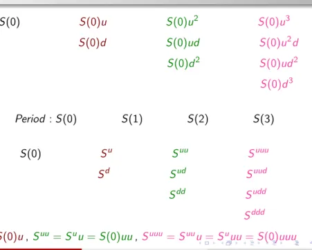
Table of Binomial Model

S(0) S(0)u S(0)u² S(0)u³

S(0)d S(0)ud S(0)u²d

S(0)d² S(0)ud² S(0)d³

Period :S(0) S(1) S(2) S(3)

S(0) S^u S^uu S^uuu

S^d S^ud S^uud

S^dd S^udd

S^ddd

One Step Binomial Model

Derivative for a risk-neutral valuation:

We set up a portfolio consisting of a long position in ∆ shares S and short position of the cash bond B. Then D = ∆S−B In the next period, the portfolio has one of two possible values:

1. ∆S^u−Be^rdt or, 2. ∆S^d−Be^rdt

We want to duplicate the values of derivatives by our portfolio as a function as

1. ∆S^u−Be^rdt =f(S^u) or, 2. ∆S^d−Be^rdt =f(S^d) The solution of ∆ andB are

∆ = f(S^u)−f(S^d)

S^u−S^d ,and B =−e^−rdt

f(S^u)− f(S^u)−f(S^d) S^u−S^d S^u

One Step Binomial Model

Since,S^u=S(0)u,S^d =S(0)d

∆ = f(S^u)−f(S^d)

S(0)(u−d) ,and B =−e^−rdt

f(S^u)−f(S^u)−f(S^d) (u−d) u

=>∆ = f(S^u)−f(S^d)

S(0)(u−d) ,and B =

df(S^u)−uf(S^d) e^−rdt(u−d)

The initial value of derivative should be the same as that of the portfolio V₀ = ∆S(0)−B, which is

D(0) = f(S^u)−f(S^d) (u−d) −

df(S^u)−uf(S^d) e^rdt(u−d)

= (f(S^u)−f(S^d))e^rdt −df(S^u) +uf(S^d) e^rdt(u−d)

One Step Binomial Model

D(0) = (e^rdt −d)f(S^u) + (u−e^rdt)f(S^d) e^rdt(u−d)

= 1

e^rdt[(e^rdt −d

u−d )f(S^u) + (1−e^rdt −d

u−d )f(S^d)]

f(S(1)) = 1

e^rdt{p_∗f(S^u) + (1−p_∗)f(S^d)}where p_∗ = e^rdt −d u−d Two cases occurs: p_∗ = ^erdt_u ^−d

−d

(i) Assume u >d, if p_∗ ≤0 then e^rdt ≤d then e^rdt ≤d <u. Then for a greened risk free profit buy stock and sell cash bound.

(ii) if p_∗ ≥ 1 then d < u ≤ e^rdt. Then for a greened risk free profit sell stock and buy cash bound.

Conclusion:

The probability of an up movement in the stock price occurs when

Two-Steps Binomial Model

In the two-steps Binomial model option expires after two time steps asS_uu, S_ud andS_dd.

Let f(S^u) andf(S^d) be the options f(S^u) = p_∗S^uu+ (1−p_∗)S^ud

e^rδt , f(S^d) = p_∗S^ud+ (1−p_∗)S^dd e^rδt

Now,

f(S(2)) = p_∗f(S^u) + (1−p_∗)f(S^d) e^rδt

= p_∗(p_∗S^uu+ (1−p_∗)S^ud) + (1−p_∗)(p_∗S^ud + (1−p_∗)S^dd) e^2rδt

= p²_∗S^uu+ 2p_∗(1−p_∗)S^ud + (1−p_∗)²S^dd e^2rδt

Multi-Steps Binomial Model

For two-steps Binomial model

D(0) =f(S(2)) = p²_∗S^uu+ 2p_∗(1−p_∗)S^ud + (1−p_∗)²S^dd e^2rδt

D(0) = f(S(1)) =e^−rdtf(S(1))

= f(S(2)) =e^−2rdtf(S(2))

= f(S(3)) =e^−3rdtf(S(3))

Multi-Steps Binomial Model

If S(1) =>single step, S(2) =>two steps,S(3) =>three steps then

f(S(1)) =p_∗f(S^u) + (1−p_∗)f(S^d)

f(S(2)) =p_∗²f(S^uu) + 2p_∗(1−p_∗)f(S^ud) + (1−p_∗)²f(S^dd) f(S(3)) =p_∗³f(S^uuu) + 3p_∗²(1−p_∗)f(S^uud) + 3p_∗(1−p_∗)²f(S^udd) +(1−p_∗)³f(S^ddd).

D(0) = ∆S(0) +B, +or − sign gives same result.

=e^−rdt{p_∗f(S^u) + (1−p_∗)f(S^d)}

=e^−2rdt{p_∗²f(S^uu) + 2p_∗(1−p_∗)f(S^ud) + (1−p_∗)²f(S^dd)}

=e^−3rdt{p_∗³f(S^uuu) + 3p_∗²(1−p_∗)f(S^uud) + 3p_∗(1−p_∗)²f(S^udd) +(1−p_∗)³f(S^ddd)}

Multi-Steps Binomial Model

V(0) = ∆S(0)−B= 1

e^rδt{pC_u+ (1−p)Cd}

= 1

e^2rδt{p²C_uu+ 2p(1−p)Cud + (1−p)²C_dd}

= 1

e^3rδt{p³C_uuu+ 3p²(1−p)Cuud+ 3p(1−p)²C_udd+ (1−p)³C_ddd

= 1

e^3rδt

3

X

j=0

3 j

p^j(1−p)^3−j(u^jd^3−jS−X)⁺.

= 1

e^nrδt

n

X

j=0

n j

p^j(1−p)^n−j(u^jd^n−jS −X)⁺.

If the price of f(0) is not equal toD(0), the arbitrage opportunity exists.

If f(0)>D(0) the trader can short the derivative (get amount of money equal tof(0)), and buy the portfolio (payD(0), and has some profit. At the expiry, the trader can sell the portfolio and buy the derivative (to return it for the short selling). Therefore, the profitf(0)−D(0) is risk-free.

Risk-Neutral valuation

We consider a portfolio consisting of a long position in ∆ shares and short position in one call, then V = ∆S −C

By no-arbitrage arguments we derive the current call option price is C₀= ∆S₀−(∆S₀u−C_u)e^−rT,

We can interpret a Risk-Neutral valuation by taking C₀=e^−rT(pCu+ (1−p)Cd)

Our subjective probability of up movement p does not appear in the final formula.

This is because V_T =K same value on up or down movement.

The value P appears in the formula and can be thought of as a probability.

Risk-Neutral valuation

We consider a portfolio consisting of a long position in ∆ shares and short position in one call, then V = ∆S −C

It is the probability implied by the market.

Fair price of a call option C₀ is equal to the expected value of its future payoff discounted at the risk-free interest rate.

For a put option P₀ (or in fact any financial contract) we have the same result P₀ =e^−rT(pPu+ (1−p)Pd).

We interpret the variable 0≤p≤1 as the probability of an up movement in the stock price. This formula is known as a risk-neutral valuation.

The probability of upp or down movement 1−p in the stock price plays no role.