Enhanced prediction of A-to-I RNA editing sites using nucleotide compositions

(1)

Enhanced prediction of A-to-I RNA editing sites using

nucleotide compositions

Ahsan Ahmad (012 173 001)

Department of Computer Science and Engineering United International University

A thesis submitted for the degree of MSc in Computer Science & Engineering

August 2019

(2)

(3)

Abstract

RNA editing process like Adenosine to Intosine (A-to-I) often influences basic functions like splicing stability and most importantly the translation.

Thus knowledge about editing sites is of great importance in molecular biology. With the growth of known editing sites, machine learning or data centric approaches are now being applied to solve this problem of prediction of RNA editing sites. In this paper, we propose EPAI-NC, a novel method for prediction of RNA editing sites. We have usedl-mer composition andn- gappedl-mer composition as features and used Pearson Correlation Coeffi- cient to select features according to Pareto Principle. Locally deep support vector machines were used to train the classification model of EPAI-NC.

EPAI-NC significantly enhances the prediction accuracy compared to the previous state-of-the-art methods when tested on standard benchmark and independent dataset.

(4)

In memory of Shuvo Bose, one of my best friends from school, died in 2016.

(5)

Published Papers

Work relating to the research presented in this thesis has been published/

submitted by the author in the following peer-reviewed journals and con- ferences:

1. Ahmad, Ahsan, and Swakkhar Shatabda. “EPAI-NC: Enhanced prediction of adenosine to inosine RNA editing sites using nucleotide compositions.” Analytical biochemistry (2019).

(6)

Acknowledgements

First of all, I would like to thank my supervisor Swakkhar Shatabda Asso- ciate Professor & Undergraduate Program Coordinator United International University for the continuous support of my research. Without his guidance it was impossible for me to complete the research and writing of this thesis.

Besides my supervisor, I wish to thank Prof. Dr. Md. Abul Kashem Mia, Professor & Dean School of Science and Engineering United International University, Prof. Dr. Mohammad Nurul Huda Professor & Director - Mas- ter of Science in Computer Science and Engineering United International University and Dr. Dewan Md. Farid Sir, Associate Professor, United In- ternational University, for critical reading of the manuscript.

This work has supported by the Department of Computer Science and En- gineering, United International University and the Business Solution De- partment, UK Department for International Development.

(7)

List of Figures

2.1 Chemical structure of DNA; hydrogen bonds shown as dotted lines .

Source [1] . . . 5

2.2 Central Dogma . . . 5

2.3 Secondary structure of a telomerase RNA. Source [2] . . . 6

3.1 Azure Tools for Machine Learning . . . 10

3.2 Sample Data . . . 11

4.1 Partiall-mers feature extraction of the first record from the Figure 3.2 20 4.2 Three Graphs (ROC, Precision vs. Recall , LIFT) of Two Class Averaged Perceptron . . . 25

4.3 Three Graphs (ROC, Precision vs. Recall , LIFT) of Two Class Bayes Point Machine . . . 27

4.4 Three Graphs (ROC, Precision vs. Recall , LIFT) of Two Class Support Vector Machine . . . 29

4.5 Three Graphs (ROC, Precision vs. Recall , LIFT) of Two Class Locally Deep Support Vector Machine . . . 31

4.6 Three Graphs (ROC, Precision vs. Recall , LIFT) of Two Class Neural Network . . . 33

4.7 Web Server Screen . . . 35

(10)

List of Tables

2.1 Summary of previous works . . . 8

3.1 Settings for Averaged Perceptron Classifier . . . 13

3.2 Settings for Two-Class Bayes Point Machine . . . 14

3.3 Settings for Two Class Support Vector Machine . . . 14

3.4 Settings for wo-Class Locally-Deep Support Vector Machine . . . 15

3.5 Settings for Two Class Neural Network Binary Classifier . . . 16

3.6 Additional columns provided by the cross validation . . . 17

3.7 Additional columns provided by the cross validation second output . . . 19

4.1 N-gapped feature extraction . . . 21

4.2 Result without feature selection at 50 % threshold . . . 22

4.3 Accuracy for different number of feature selected at 50 % threshold for our selected algorithms . . . 23

4.4 Result of Averaged Perceptron Classifier . . . 24

4.5 Result of Two-Class Bayes Point Machine . . . 26

4.6 Result of Two Class Support Vector Machine . . . 28

4.7 Result of wo-Class Locally-Deep Support Vector Machine . . . 30

4.8 Results of Two Class Neural Network Binary Classifier . . . 32

4.9 Jackknife Test comparison . . . 34

4.10 Comparison with other methods . . . 34

4.11 Comparison with other methods based on Independent dataset . . . 35

(11)

Chapter 1

Introduction

The process of RNA editing takes place when a genomic template passes through transcription. In this process nucleotides are modified in the genomic template and turns into a different one[3]. RNA editing creates diversity in species. The common modifications includes, Cytidine to Uridine (C to U), Adenosine to Inosine (A to I), non- templated nucleotide additions and insertions and so on. The amino acid sequence in mRNAs are changed because of RNA editing [4]. The basic functions like splicing, stability, localization, and translation of mRNA are highly influenced by A-to-I editing[5].

Among the post transcriptional processes of RNA, editing is important which also bring changes in gene expression. In terms of A-to-I RNA editing, it has major impact in human gene functions. [6]. Currently ‘Comparison of cDNA sequences’ is the widely used method for identifying A-to-I editing chemically [7] [8]. Inosine(hypoxanthine)-cytidine (I-C) is one of the four main wobble base-pairs. A site will be a candidate of A-to-I editing if, in the process of reverse-transcription and PCR inosines (I) are modified to guanosines (G) in the cDNA. This process is also known as RNA–DNA differences (RDDs)[9][10][11]. Though this method has high accuracy, this is an expensive and time consuming method. As the amount of discovering RNA sequences has increased, there is a high demand to develop computational methods to help the scientists to get the information[12].

(12)

1.1 Motivation

In the last decade with the huge growth biological data systems biology becomes the most interesting section in the field of molecular research.

A particular type of RNA editing called adenosine to inosine (A-to-I) RNA plays a key role in protein variation in cancer cells. In the transcription phase when mRNA carries the information from DNA to ribosome sometimes the genetic informations got altered this process is known as RNA editing.

1.2 Objectives of the Thesis

From our observation of other thesis work we believe that the accuracy of the other predictors can be enhanced and also it is possible to build better tools for the scientists.

Also we didn’t find any thesis work that has used Microsoft’s Azure Machine Learn- ing Studio. So we also want to experiment if we can use this platform for bioinformatics.

So here is the objectives we want to cover in this thesis work:

• Enhance the accuracy of the algorithm.

• Build a better web based tool to predict adenosine to inosine (A-to-I) RNA editing.

• Use Azure Machine Learning Studio (Azure ML) for bioinformatics.

1.3 Thesis Contributions

Here in this work, we enhance our prediction model by generating a bigger number of feature extraction and selecting important number of features using two basic algorithms. So from the algorithm point of view the model is simple yet powerful to predict A-to-I editing site more accurately.

As, we are using Azure ML Studio for our experiment, it opens a wide range of opportunity to go for more complex experiments with less difficulties.

(13)

1.4 Organization of the Thesis

The thesis are divided into 5 chapters. We are now in Chapter 1 which contains Declaration,Certificate, Abstract,Acknowledgments, the Table of Contents and Introduction. Other chapters are designed as follows:

Chapter 2 provides brief idea about background works related to the work that inspired me to work with this topic.

Chapter 3 describes the Azure environment we would like to explore, the dataset, feature extraction and selection. Finally, the selective five algorithms that gives the best result on the dataset we prepare.

Chapter 4 shows the result we got from our experiments and finally the result we want to stop for the time being.

Chapter 5 presents the conclusions, summaries the thesis contributions, and discusses the future works.

(14)

Chapter 2

Background Analysis

2.1 Introduction

In this chapter we describe the biological and computational background of our work.

2.2 Biological Background

Any living beings are made of cells. Each cell of an organism contains a full set of instructions to build and maintain. This set of instructions is known as genome. Similar cells, e.g., kidney cells, contain same set of instructions.

These set of instructions are made of deoxyribonucleic acid(DNA). DNA is the blue print of making proteins in living body.

DNA is a combination of molecules known as nucleotides. Each nucleotide has a phosphate group, a sugar group and a nitrogenous base. Only four types of nitrogenous bases are used for building DNA. These are Adenine(A), Thymine (T), Guanine (G) and Cytosine (C).

(15)

2.2 Biological Background

Figure 2.1: Chemical structure of DNA; hydrogen bonds shown as dotted lines . Source [1]

So we know that necessary proteins are generated according to DNA instructions.

The process is known as Central Dogma. The basic idea of central dogma is: a flow of genetic information through RNA from DNA for creating a protein.

Figure 2.2: Central Dogma

RNA is assembled as a chain of nucleotides to convey message. It consists of adenine (A), cytosine (C), guanine (G), and uracil (U) nucleobases. There are several kind of RNAs.

(16)

2.2 Biological Background

Figure 2.3: Secondary structure of a telomerase RNA. Source [2]

Among them most important types are Messenger RNA (mRNA): works for conveying genetic information andTransfer RNA (tRNA):helps the process of protein synthesis. Many viruses encode their genetic information using an RNA genome.

Though we have idea about central dogma, we might has shallow knowledge about the changes to mRNA that occur after transcription. Some nuclease are altered in the mRNA; is known as RNA editing.

RNA editing is the process by which ribonucleic acid (RNA) molecules are enzy- matically modified post synthesis on specific nucleosides. There are two ways of RNA editing: addition, by which new nucleotides are inserted into the original sequence and deletion, or removal of a nucleotide, can also cause a frameshift.

There are two types of RNA editing occurs by deamination: C-to-U editing: the process of changing a cytidine base into a uridine base, and A-to-I editing: the process of adenosine (A) turns to inosine (I). Inosine is then decoded as guanosine (G) in translation. Among the types of RNA editing, A-to-I editing is the regular event done by double-stranded RNA-specific adenosine deaminase (ADAR) enzymes.

(17)

2.3 Computational Background

This kind of modifications directly effects the functionality and stability of the RNA.

Sometime it causes good modifications but most of the time it creates diseases. Several kind of cancers are introduced by this kind of editing. However, some current studies found that this kind of editing commonly takes place in non-coding area of the genome which has major implications for evolution and creating diseases.[13]

2.3 Computational Background

In brief, prediction of attributes or functions biological sequences are modelled as binary classification problem which uses supervised machine learning algorithms. In the last couple of years, several studies have been done to predict attributes or functions that covers proteins [14, 15], DNA [16, 17] and RNA sequences [18, 19]. For feature extraction various techniques are being used. The most important one is the PseAAC [20] which was built for protein sequences initially but extended for DNA and RNA sequences as well [21]. Other successful feature extraction methods that are evolutionary [22], hidden markov model [23], structural [24] and pysicho-chemical features [15].

Several successful supervised machine learning algorithms has been used in the litera- ture: Support Vector Machines [24], Logistic Regression [17], AdaBoost Algorithm [25], Artificial Neural Networks [26], etc.

For eternity, among the computational biologists, RNA editing is an attractive topic[27–30]. A number of studies have been done where the computational biologists had used machine learning to address A-to-I prediction. In 2013, St Laurent et al.

proposed a model to identify A-to-I editing sites in D. melanogaster using an inter- active feedback loop. But this study has no usable tools provided[31]. In 2016, Chen et al proposed another prediction model titled “PAI” with is based on support vector machine. A web based tool had constructed to use this model [18]. In the year 2017, another predictor is proposed titled “iRNA-AI” which is also based on support vector machine. Though this paper used a different dataset [19]. Later on, Xiao et al tried to enhance the accuracy of identifying A-to-I RNA editing [12] based on the dataset used in “PAI”. The method they proposed was called “PAI-SAE”. Prediction of RNA editing site problems and prediction of post translational modification (PTM) site problems

(18)

are very similar. For solving the PTM prediction problem, several supervised learning based methods have been proposed [15, 32–43].

So the following table summarizes major works done in recent days Table 2.1: Summary of previous works

Name Dataset Features Algorithm(s) Accuracy

over benchmark data Effective DNA

binding protein prediction by using key features via Chou’s general PseAAC

Berman, H. M.

et al. The protein data bank [44]

Monogram, Bi- gram, Trigram, Gapped bigram, Monogram percentile, Bigram percentile, Near- est neighbor bigram

Extra Tree Classifier and Random Forest

95.91 %

iRSpot-SF: Pre- diction of recombination hotspots by incorporating sequence based features into Chou’s Pseudo components

standard benchmark datasets

Gapped k-mer composition and reverse com- plement k-mer composition

SVM with

RBF kernel

84.58 %

PAI: Predicting adenosine to inosine editing sites by using pseudo nucleotide compositions

wild-type D.

melanogaster

Pseudo dinu- cleotide composition

Support Vec- tor Machine

79.51 %

In the work presented here, we propose an enhanced support vector machine (SVM) based-method to identify the A-to-I editing site in D. melanogaster analyze the RNA sequence by extracting different features (e.g. l-mar and n-gapped) in the RNA se-

(19)

quence. Also we build a web server http://epai-nc.info, by which anyone can use the proposed model easily.

(20)

Chapter 3

Materials and Methods

This is clearly difficult to predict a situation when it is related to biological element.

We have started from collecting a good dataset to achieve this task. Then we extracted features from the dataset then find out the most correlated features with the target concerned level. Then we implement some classification algorithm and found that Support Vector Machine gives the best output.

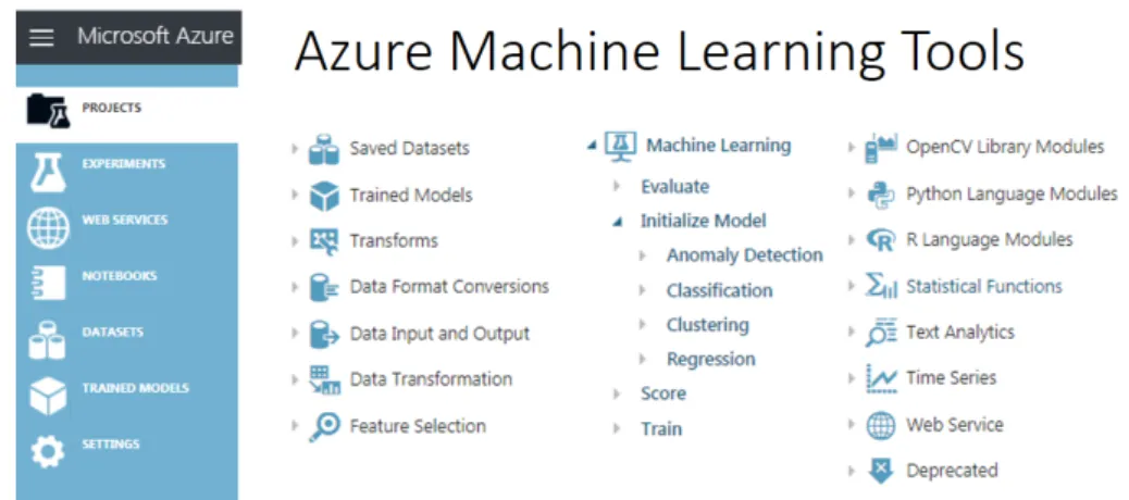
3.1 Azure Machine Learning Studio

In this work we use Microsoft’s Azure Machine Learning Studio https:// studio.azureml.net/

for the very first time for experimenting bioinformatics related experiment.

Figure 3.1: Azure Tools for Machine Learning

(21)

3.2 Dataset

The reason behind using this tool is pretty straight forward. This tools has the following features that are one of its kind so far.

• This tool is cloud based so we do not need to set up any software in our local machine.

• As the tool is cloud based we do not tension about running long process in local machines which may interrupt by bad network connection or discontinuity of electricity

• It is easy to share. Also it has built-in features to build shareable web API for farther development or integrated to excel.

• This tool has built-in interface to collect data from different kind of data sources so it is very easy to incorporate with any exiting system without altering any exiting hardware.

3.2 Dataset

We obtained the dataset form ‘http://lin.uestc.edu.cn/server/PAI’ which is the official website for the paper “PAI: Predicting adenosine to inosine editing sites by using pseudo nucleotide compositions”[18]. There were two different kind of dataset: i) benchmark and ii) independent.

3.2.1 Benchmark Dataset

Figure 3.2: Sample Data

The benchmark dataset contains the RNAs of the D. melanogaster, which is pre- pared for carrying out genome-wide studies of adenosine-to-inosine RNA editing with

(22)

3.3 Feature Extraction

single molecular sequencing [31]. It contains, S, 244 sets of sample RNA sequences.

Among them, S⁺, 125 items are actually contains A-to-I modification and other, S^-, 119 items are not. So the total dataset can be formulated as follows:

S=S⁺∪S⁻

, (3.1)

where∪represents union of the subsets.

Each sequence contains 51 nucleotides. Each record consists of two rows: the first row contains positive/negative identifier and the second row contains the RNA sequence. Each sequence is made of four letters (A,G,C,U). They stands for Adenine - A, Guanine - G, Cytosine - C and Uracil - U.

3.2.2 Independent Dataset

From Yu and his colleagues’ work[45], an independent dataset is generated by harvesting A-to-I editing site containing sequences of D. melanogaster to test the strength of proposed method. The Independent dataset contains 300 records. Each record also contains 51 nucleotides that all are true candidate of A-To-I modification.

3.3 Feature Extraction

Feature extraction is the very first process of our experiment. Here, the target is to generate as much as features possible from the nucleotide sequences. So that we can analyze the sequence as a whole. Finally we get 92820 features extracted.

3.4 Feature Selection

After extracting features we run some selective algorithms to understand the strength of algorithms over the features. The results are good but not that much promising.

Also we found that all features are not that much important for the prediction model.

So we are approaching to run feature selection. We used Pearson Correlation algorithm to find the best related features. And proceed keeping Pareto principle (80-20

(23)

3.5 Algorithms

rule) in our mind for determining the number of features we should take for this model.

Finally we choose first 20000 features for our experiment.

3.5 Algorithms

In Azure Machine Learning Studio, there are some built-in algorithms for classification.

We choose all of the algorithms for the experiment but get good result for the following algorithms.

3.5.1 Averaged Perceptron Classifier

This is a very simple version of neural network and this is a supervised learning algorithm. This method uses a linear function to classify inputs into several possible outputs merged with a weight which is derived from the feature vector. That’s why this is called “perceptron”.

To run this algorithm we used following settings.

Table 3.1: Settings for Averaged Perceptron Classifier

Setting Value

Initial Learning Rate 0.001 Maximum Number Of Iterations 50

Batch Size 256

Learning Rate Decay Exponent 0.5

Averaging Weight 0.5

Tolerance 1.00E-05

Allow Unknown Levels TRUE

Random Number Seed 123

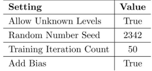
3.5.2 Two-Class Bayes Point Machine

This method is based on Bayesian process for linear classification. Theoretically, this method approximates the optimal Bayesian average of a linear classifier efficiently.

(24)

3.5 Algorithms

For experimenting our dataset using this algorithm our parameter values were like below.

Table 3.2: Settings for Two-Class Bayes Point Machine

Setting Value

Allow Unknown Levels True Random Number Seed 2342 Training Iteration Count 50

Add Bias True

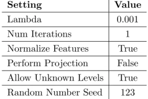
3.5.3 Two-Class Support Vector Machine

For both classification and regression Support vector machine or SVM is an powerful algorithm. This method can classify linear and non-linear tasks. This is a supervised learning model which takes labeled data for learning. During the training process this algorithm organizes input data points in the hyperplane - a multi-dimensional feature space. Which divides the output categories as wide as possible.

For Two-Class Support Vector Machine the settings were like below.

Table 3.3: Settings for Two Class Support Vector Machine

Setting Value

Lambda 0.001

Num Iterations 1

Normalize Features True Perform Projection False Allow Unknown Levels True Random Number Seed 123

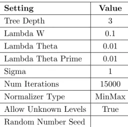
3.5.4 Two-Class Locally-Deep Support Vector Machine

This is an own implementation of Microsoft Research to speed up non-linear SVM prediction. In this implementation, the base function is redesigned to mapping data points

(25)

3.5 Algorithms

to the feature space. This reduces the time of training maintaining the classification accuracy.

Following is the settings we used for running this algorithm. And this is the best one that gives the best outcome for the independent dataset.

Table 3.4: Settings for wo-Class Locally-Deep Support Vector Machine

Setting Value

Tree Depth 3

Lambda W 0.1

Lambda Theta 0.01

Lambda Theta Prime 0.01

Sigma 1

Num Iterations 15000

Normalizer Type MinMax Allow Unknown Levels True Random Number Seed

3.5.5 Difference Between SVM and LD-SVM

This method uses the localized multiple kernel learning method developed by Gonen and Alpaydin in 2008 [46]. Using this method helps LD-SVM to learn embedded local features having high-dimensional, sparse, and computationally deep features of a non- linear model

Following are the important reasons that make LD-SVM faster:

• This method can test a new point against its local decision boundary.

• By using primal-based routines this method reduce the required space.

3.5.6 Two Class Neural Network Binary Classifier

Neural Network or artificial neuron network (ANN) is another machine learning algorithm that can be supervised or unsupervised. Two Class Neural Network Binary

(26)

3.5 Algorithms

Classifier is a supervised version. The work flow and the structure of this method is inspired by the biological neural networks. Two Class Neural Network consists of two or more interconnected layers: the first layer is the input layer and the last layer is the output layer. Between these two layers we can add multiple hidden layers. By default, it uses sigmoid function as activation function for classification models. This algorithm is highly customizable. for customizing we have to use Net# language developed at Microsoft by Shon Katzenberger (Architect, Machine Learning) and Alexey Kamenev (Software Engineer, Microsoft Research).

For Neural Network Binary Classifier settings value was like below.

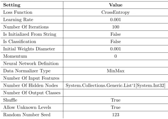
Table 3.5: Settings for Two Class Neural Network Binary Classifier

Setting Value

Loss Function CrossEntropy

Learning Rate 0.001

Number Of Iterations 100

Is Initialized From String False

Is Classification False

Initial Weights Diameter 0.001

Momentum 0

Neural Network Definition

Data Normalizer Type MinMax

Number Of Input Features

Number Of Hidden Nodes System.Collections.Generic.List‘1[System.Int32]

Number Of Output Classes

Shuffle True

Allow Unknown Levels True

Random Number Seed 123

(27)

3.6 Performance Evaluation

For evaluating the performance of our models, we used k-Fold Cross-Validation with k

= 10. For doing so AzureML has a dedicated built-in feature calledCross-Validation Model.

3.6.1 Cross-Validation Model

Input: A labeled dataset and an untried classification or regression model.

Output: A set of accuracy statistics for each fold:

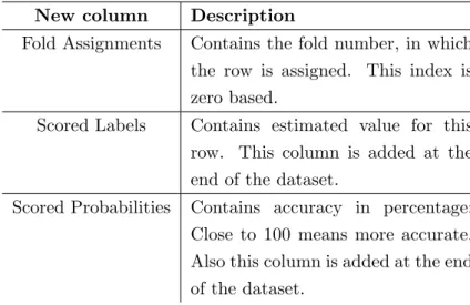
Table 3.6: Additional columns provided by the cross validation

New column Description

Fold Assignments Contains the fold number, in which the row is assigned. This index is zero based.

Scored Labels Contains estimated value for this row. This column is added at the end of the dataset.

Scored Probabilities Contains accuracy in percentage;

Close to 100 means more accurate.

Also this column is added at the end of the dataset.

Processing Method: By default, this model divides the input dataset into 10 subsets or folds. Then uses 9 folds for training and 1 fold for validating, and repeat this process for all folds.

3.6.2 Evaluation results by fold

To understand the formulas of “Evaluation results by fold” records, we have to know some other basics.

(28)

• True Positives (TP)- Number of correctly identified positive records.

• True Negatives (TN)- Number of correctly identified negative records.

• False Positives (FP)- Number of incorrectly identified positive records.

• False Negatives (FN)- Number of incorrectly identified negative records.

Following is the set of figures we get from Cross Validation Model.

That is evaluation results by fold. This contains (number of folds + 2) rows of records.

Additionally, the following metrics are included for each fold for Classification models: Precision, Recall, F-score, AUC.

(29)

Table 3.7: Additional columns provided by the cross validation second output

Column name Description

Fold number This is 0 based indexing. If the analysis have 10 folds then the value of this column will be 0 to 9, ‘Mean’

and ‘Standard Deviation’

Number of examples in fold This figure shows how many rows from the dataset assigned in a particuler fold. This figure is roughly equal through all rows

Model Shows the name of the algorithm that process the fold Accuracy Is the ratio of correctly identified and all records

T P +T N/T P+F P +F N +T N

Precision Is the ratio of truly positive and all positive records T P/T P +F P

Recall Also known as sensitivity. Is the ratio of identified true positive and all true positive record

T P/T P +F N

F-Score 2*(Recall * Precision) / (Recall + Precision)

AUC Area under (the ROC) Curve. whereas “Accuracy”

defines a result as true or false “AUC” provides a threshold to define the “True” and the “False”.

(30)

Chapter 4

Experimental Analysis

In this chapter we discuss the elaborated results we obtained throughout the experiment and the final result we have picked from all of them.

4.1 Result of Feature Analysis

To achieve that, first we have extractedl-mers up to 6-mers or (2 codon length)-mers.

so we get total 5460 features.

4¹+ 4²+ 4³+ 4⁴+ 4⁵+ 4⁶= 5460 (4.1)

Figure 4.1: Partiall-mers feature extraction of the first record from the Figure 3.2

(31)

4.1 Result of Feature Analysis

Then we implemented the n-gapped feature extraction. We keep same number of nucleotides in both side of the gap. We increased up to 21 gaps having up to 3 nucleotides on both sides. So we get around 91728 features. The breakdown is like below:

Table 4.1: N-gapped feature extraction

Number of Gap

Sample Number

of Fea- tures 1-gapped A.A, A.C, . . . , AC.AC, CC.CC, . . . ,AAA.AAA,

AAA.AAC, . . .

4368 2-gapped A..A, A..C, . . . , AC..AC, CC..CC, . . . ,AAA..AAA,

AAA..AAC, . . .

4368 3-gapped A...A, A...C, . . . , AC...AC, CC...CC, . . .

,AAA...AAA, AAA...AAC, . . .

4368

... ... ...

19-gapped A...A, . . . , AC...AC, . . . ,AAA...AAA, . . .

4368 20-gapped A...A, . . . , AC...AC, . . .

,AAA...AAA, . . .

4368

Total Number of features 87360

We can represent it like the following equation

4368×20 = 87360 (4.2)

Here is the breakdown of 4368 features of the each gap.

4²+ 4⁴+ 4⁶= 4368 (4.3)

By equations 4.1 and 4.2, the total number of features is

87360 + 5460 = 92820 (4.4)

(32)

4.1.1 Feature Selection

After getting so many features we have approached to test our selected algorithms on generated features and good progress for all of the algorithms.

Table 4.2: Result without feature selection at 50 % threshold

Algorithm Accuracy Precision Recall F1 Score AUC Two-Class Averaged

Perceptron

0.816 0.774 0.904 0.834 0.874

Two-Class Bayes Point Machine

0.803 0.755 0.912 0.826 0.801

Two-Class Locally- Deep Support Vec- tor Machine

0.779 0.735 0.888 0.804 0.866

Two-Class Neural Network

0.811 0.765 0.912 0.832 0.869

Two-Class Support Vector Machine

0.770 0.752 0.824 0.786 0.870

But we have also found that all the features are not significant for predicting A-to-I RNA Editing. So we decided to select top around 20 % features according to Pareto principle. As this method estates that we should get a good result(80 % good) from 20% features, that is 18564 features. So we run our experiment taking 15000, 18000, 19000, 20000, 21000, 22000 and found that having 20000 features we are getting best sets of accuracy.

(33)

Table 4.3: Accuracy for different number of feature selected at 50 % threshold for our selected algorithms

Number of Fea- tures

Support Vector Machine

Averaged Percep- tron

Bayes Point Machine

Locally- Deep Support Vector Machine

Neural Network

15000 0.926 0.918 0.984 0.910 0.898

18000 0.930 0.926 0.988 0.930 0.910

19000 0.930 0.926 0.992 0.926 0.898

20000 0.934 0.926 0.992 0.930 0.898

21000 0.930 0.922 0.992 0.934 0.910

22000 0.918 0.926 0.992 0.926 0.902

So we take best 20000 features for further experiment. For selecting best features we have used Pearson correlation.

(34)

4.2 Algorithm wise results

While experimenting with a range of algorithms, following five algorithms give the best results. For all these algorithms we have picked resultant values at the 30%, 50% and 70% thresholds to compare the wellness of the models.

4.2.1 Averaged Perceptron Classifier

This method is best for training linearly separable patterns. As perceptrons process scenarios serially, this is faster than a complex neural network. So using this algorithm we get the follwoing results at different threshold.

Table 4.4: Result of Averaged Perceptron Classifier

Thres- hold

True Pos- itive

False Neg- a- tive

False Pos- itive

True Neg- a- tive

Accu- racy

Preci- sion

Re- call

F1 Score

AUC

0.3 124 1 21 98 0.910 0.855 0.992 0.919 0.987

0.5 120 5 11 108 0.934 0.916 0.96 0.938 0.987

0.7 114 11 4 115 0.939 0.966 0.912 0.938 0.987

And this is the ROC, Precision vs. Recall , LIFT Graphs for this method.

(35)

Figure 4.2: Three Graphs (ROC, Precision vs. Recall , LIFT) of Two Class Averaged Perceptron

(36)

4.2.2 Two-Class Bayes Point Machine

This method is a Bayesian classification model, it is not suffer from over fitting problem while training the data. Following are the results we got at different threshold for this algorithm.

Table 4.5: Result of Two-Class Bayes Point Machine

Thres- hold

True Pos- itive

False Neg- a- tive

False Pos- itive

True Neg- a- tive

Accu- racy

Preci- sion

Re- call

F1 Score

AUC

0.3 125 0 77 42 0.684 0.619 1 0.765 0.995

0.5 123 2 0 119 0.992 1 0.984 0.992 0.995

0.7 18 107 0 119 0.561 1 0.144 0.252 0.995

And below is the ROC, Precision vs. Recall , LIFT graphs we got.

(37)

Figure 4.3: Three Graphs (ROC, Precision vs. Recall , LIFT) of Two Class Bayes Point Machine

(38)

4.2.3 Two-Class Support Vector Machine

This is also known support vector networks or SVN. this is another supervised learning algorithm that divides the data into two section.

Using SMV we got the following results on benchmark data.

Table 4.6: Result of Two Class Support Vector Machine

Thres- hold

True Pos- itive

False Neg- a- tive

False Pos- itive

True Neg- a- tive

Accu- racy

Preci- sion

Re- call

F1 Score

AUC

0.3 124 1 21 980 0.910 0.855 0.992 0.919 0.987

0.5 120 5 11 108 0.934 0.916 0.960 0.938 0.987

0.7 114 11 4 115 0.939 0.966 0.912 0.938 0.987

And here goes the ROC, Precision vs. Recall , LIFT graphs for this algorithm

(39)

Figure 4.4: Three Graphs (ROC, Precision vs. Recall , LIFT) of Two Class Support Vector Machine

(40)

4.2.4 Two-Class Locally-Deep Support Vector Machine (LD-SVM) This method is optimized in such ways that it can work with larger training sets more efficiently. This is a fully supervised learning algorithm. This method can give quick prediction than both Non-linear and linear classifiers though it compromises classification accuracies a bit.

Using LD-SVM the result we got as follows:

Table 4.7: Result of wo-Class Locally-Deep Support Vector Machine

Thres- hold

True Pos- itive

False Neg- a- tive

False Pos- itive

True Neg- a- tive

Accu- racy

Preci- sion

Re- call

F1 Score

AUC

0.3 120 5 20 99 0.898 0.857 0.960 0.906 0.984

0.5 120 5 12 107 0.930 0.909 0.960 0.934 0.984

0.7 115 10 9 110 0.922 0.927 0.920 0.924 0.984

And the graphs are like below.

(41)

Figure 4.5: Three Graphs (ROC, Precision vs. Recall , LIFT) of Two Class Locally Deep Support Vector Machine

(42)

4.2.5 Two Class Neural Network Binary Classifier

For computing the output, at each node of the hidden layers and output layer that value is calculated. This value is calculating from the weighted sum of the values from the previous layer. Also an activation function take place to calculate that weighted sum.

So the output of this algorithm on benchmark data is:

Table 4.8: Results of Two Class Neural Network Binary Classifier

Thres- hold

True Pos- itive

False Neg- a- tive

False Pos- itive

True Neg- a- tive

Accu- racy

Preci- sion

Re- call

F1 Score

AUC

0.3 122 3 32 87 0.857 0.792 0.976 0.875 0.975

0.5 117 8 19 100 0.889 0.860 0.936 0.897 0.975

0.7 111 14 7 112 0.914 0.941 0.888 0.914 0.975

So as the graphs are:

(43)

Figure 4.6: Three Graphs (ROC, Precision vs. Recall , LIFT) of Two Class Neural Network

(44)

4.3 Jackknife Test

So after doing all those experiments we found thatSupport Vector Machine,Aver- aged Perceptron, Locally-Deep Support Vector Machine give good accuracies over 10-fold cross validation. The values are 93.4%, 93.4%, 93% respectively. So we then decide to run Jackknife Test on benchmark dataset using all these algorithms and finally we got the following results:

Table 4.9: Jackknife Test comparison

Model Algorithm ACC (%) Jackknife Test (%)

Support Vector Machine 93.4 92.2

Averaged Perceptron 93.4 93

Locally-Deep Support Vector Machine 93 93.9

4.4 Final Results

Based on the result of Jackknife test we finally decide to pick the Locally-Deep Support Vector Machine algorithm as the selected one for building our prediction model.

4.4.0.1 On benchmark data

Listed in the following table are the comparison of EPAI-NC with the other predictor like PAI-SAE and PAI via jackknife test on benchmark dataset for identifying A-to-I editing sites inD. melanogaster.

Table 4.10: Comparison with other methods

Predictor ACC (%) MCC (%) Sn (%) Sp (%)

PAI 79.51 60.00 85.60 73.11

PAI-SAE 81.97 64.14 87.20 76.47

EPAI-NC 93.90 87.90 96.80 90.80

(45)

4.5 Web Server

4.4.0.2 On independent data

Also we have tested our proposed model against the independent dataset to see how much site it can Identify. In this test, our proposed model gives better result than PAI also.

Table 4.11: Comparison with other methods based on Independent dataset

Predictor Correctly Identified Site ACC (%)

PAI 247 82.33

PAI-SAE No data Found No data Found

EPAI-NC 253 84.33

4.5 Web Server

For the convenience of scientific community, we also develop a freely accessible web based application. To use this application please follow the following steps.

Figure 4.7: Web Server Screen

(46)

4.5 Web Server

4.5.1 The Application

The address of our application is http://epai-nc.info/. You will get the main page of the application which contains a big text box and a button titled ‘Predict’. To use this application you have to give a valid RNA site as input and click Predict button.

4.5.2 The Input

To get the best result you have to give any RNA string having minimum length of 51 bp. there is no maximum length limit.

Sample Input 1:

AAAGGUUUCCUUGGUCACGUUCGCCACUUACGUGCUAACCAGCGAGGCGAA Sample Input 2 (without -):

ACUGAAAGAAGGGAUUGAACUGUUUAGACCCAAAUCGAUCGCCAAUUAUAC- AUAGUAAUCUGCCCGAGAGUUGCUGGGACACGAUAUGCAACAAAUAGGUGA- CUAAAAUAUUCCAUUAAAGUAAAAUAUUCCACCCAAGCAAUUAGAAAUCGU- ACAUUUAAGGGCUGGCUAUAAUAUACGGAAAUUUGUUUUUUUUUU

4.5.3 The Output

After clicking the “Predict” button the application returns a set of positions of A’s and the probabilities of being edited in percentage. If the parentage of the probability close to 100% then it is more likely a good candidate of Editing. on the other hand if it is close to 0% this may not be edited.

(47)

Chapter 5

Conclusion

5.1 Summary

Identification of adenosine-to-inosine editing sites play a vital role in identifying cancer, this may also be the key feature for understanding the non-coding part of the RNA sequences. In this study we constructed a new predictor for identifying A-to-I modification which is simplified from the previous methods. Also as we get best result for benchmark data. This gives us confidence to say that our predictor is currently the best one and can easily be used as an analytic solution to more genomic problems.

5.2 Limitation

Important to mention, as we have selected a big number of features, the model could be prone to over fitting. However, further optimize is possible by using similar techniques used in [47, 48]. Also, we would like to use chemical properties of nucleotides which are proven techniques to solve related problems [49, 50].

5.3 Future Work

So far what we get is based on onlyD. melanogaster. In future one may try to find out how it behaves for other datasets collected from other species. Also, in future, one may try to develop a deep learning-based framework to precisely and conveniently predict RNA editing sites using RNA-seq data alone which may include ensemble learning.

(48)

5.3 Future Work

Also one may try to use this same model to identify the location of RNA that are going to be edited.

(49)

Bibliography

[1] Madprime. Dna chemical structure. https://commons.wikimedia.org/wiki/File:

DNA chemical structure.svg. ix, 5

[2] Narayanese. (2007, Nov..) Ciliate telomerase rna. https://commons.wikimedia.

org/wiki/File:Ciliate telomerase RNA.JPG. ix, 6

[3] S.-J. Cho, V. Blanc, and N. O. Davidson, “Mouse models as tools to explore cytidine-to-uridine rna editing,” vol. 424, pp. 417–435, 2007. 1

[4] A. Brennicke, A. Marchfelder, and S. Binder, “Rna editing,” FEMS Microbiology Reviews, vol. 23, no. 3, pp. 297–316, 1999. [Online]. Available:

http://dx.doi.org/10.1111/j.1574-6976.1999.tb00401.x 1

[5] D. Fumagalli, D. Gacquer, F. Roth´e, A. Lefort, F. Libert, D. Brown, N. Khed- doumi, A. Shlien, T. Konopka, R. Salgado et al., “Principles governing a-to-i rna editing in the breast cancer transcriptome,” Cell reports, vol. 13, no. 2, pp. 277–

289, 2015. 1

[6] W. Tang, Y. Fei, and M. Page, “Biological significance of rna editing in cells,”

Molecular biotechnology, vol. 52, no. 1, pp. 91–100, 2012. 1

[7] C. M. Burns, H. Chu, S. M. Rueter, L. K. Hutchinson, H. Canton, E. Sanders- Bush, and R. B. Emeson, “Regulation of serotonin-2c receptor g-protein coupling by rna editing,” Nature, vol. 387, no. 6630, p. 303, 1997. 1

[8] N. Paz, E. Y. Levanon, N. Amariglio, A. B. Heimberger, Z. Ram, S. Constantini, Z. S. Barbash, K. Adamsky, M. Safran, A. Hirschberg et al., “Altered adenosine- to-inosine rna editing in human cancer,” Genome research, vol. 17, no. 11, pp.

000–000, 2007. 1

(50)

BIBLIOGRAPHY

[9] M. Li, I. X. Wang, Y. Li, A. Bruzel, A. L. Richards, J. M. Toung, and V. G. Che- ung, “Widespread rna and dna sequence differences in the human transcriptome,”

science, p. 1207018, 2011. 1

[10] J. H. Bahn, J.-H. Lee, G. Li, C. Greer, G. Peng, and X. Xiao, “Accurate identification of a-to-i rna editing in human by transcriptome sequencing,” Genome research, 2011. 1

[11] Z. Peng, Y. Cheng, B. C.-M. Tan, L. Kang, Z. Tian, Y. Zhu, W. Zhang, Y. Liang, X. Hu, X. Tan et al., “Comprehensive analysis of rna-seq data reveals extensive rna editing in a human transcriptome,” Nature biotechnology, vol. 30, no. 3, p.

253, 2012. 1

[12] X. Xiao, P. Wang, Z. Xu, W. Qiu, and X. Fang, “Pai-sae: Predicting adenosine to inosine editing sites based on hybrid features by using spare auto-encoder,” in IOP Conference Series: Earth and Environmental Science, vol. 170, no. 5. IOP Publishing, 2018, p. 052018. 1, 7

[13] E. Eisenberg and E. Y. Levanon, “A-to-i rna editing—immune protector and transcriptome diversifier,” Nature Reviews Genetics, p. 1, 2018. 7

[14] S. Adilina, D. M. Farid, and S. Shatabda, “Effective dna binding protein prediction by using key features via chou’s general pseaac,” Journal of theoretical biology, 2018. 7

[15] M. M. Islam, S. Saha, M. M. Rahman, S. Shatabda, D. M. Farid, and A. De- hzangi, “iProtGly-SS: identifying protein glycation sites using sequence and structure based features,” Proteins: Structure, Function, and Bioinformatics, 2018. 7, 8

[16] M. A. Al Maruf and S. Shatabda, “iRSpot-SF: Prediction of recombination hotspots by incorporating sequence based features into chou’s pseudo components,”Genomics, 2018. 7

[17] M. R. Jani, M. T. K. Mozlish, S. Ahmed, N. S. Tahniat, D. M. Farid, and S. Shatabda, “iRecSpot-EF: Effective sequence based features for recombination hotspot prediction,” Computers in biology and medicine, 2018. 7

(51)

BIBLIOGRAPHY

[18] W. Chen, P. Feng, H. Ding, and H. Lin, “Pai: Predicting adenosine to inosine editing sites by using pseudo nucleotide compositions,” Scientific reports, vol. 6, p. 35123, 2016. 7, 11

[19] W. Chen, P. Feng, H. Yang, H. Ding, H. Lin, and K.-C. Chou, “irna-ai: identifying the adenosine to inosine editing sites in rna sequences,” Oncotarget, vol. 8, no. 3, p. 4208, 2017. 7

[20] P. Du, X. Wang, C. Xu, and Y. Gao, “PseAAC-Builder: A cross-platform stand- alone program for generating various special chou’s pseudo-amino acid compositions,” Analytical biochemistry, vol. 425, no. 2, pp. 117–119, 2012. 7

[21] W. Chen, T.-Y. Lei, D.-C. Jin, H. Lin, and K.-C. Chou, “PseKNC: a flexible web server for generating pseudo k-tuple nucleotide composition,” Analytical biochemistry, vol. 456, pp. 53–60, 2014. 7

[22] S. Y. Chowdhury, S. Shatabda, and A. Dehzangi, “iDNAProt-ES: Identification of dna-binding proteins using evolutionary and structural features,” Scientific Re- ports, vol. 7, no. 1, p. 14938, 2017. 7

[23] R. Zaman, S. Y. Chowdhury, M. A. Rashid, A. Sharma, A. Dehzangi, and S. Shatabda, “HMMBinder: Dna-binding protein prediction using hmm profile based features,” BioMed research international, vol. 2017, 2017. 7

[24] S. Shatabda, S. Saha, A. Sharma, and A. Dehzangi, “iPHLoc-ES: Identification of bacteriophage protein locations using evolutionary and structural features,”

Journal of theoretical biology, vol. 435, pp. 229–237, 2017. 7

[25] F. Rayhan, S. Ahmed, S. Shatabda, D. M. Farid, Z. Mousavian, A. Dehzangi, and M. S. Rahman, “iDTI-ESBoost: Identification of drug target interaction using evolutionary and structural features with boosting,”Scientific reports, vol. 7, no. 1, p. 17731, 2017. 7

[26] F. Rayhan, S. Ahmed, Z. Mousavian, D. M. Farid, and S. Shatabda, “FRnet- DTI: Convolutional neural networks for drug-target interaction,” arXiv preprint arXiv:1806.07174, 2018. 7

(52)

BIBLIOGRAPHY

[27] J. Sun, Y. De Marinis, P. Osmark, P. Singh, A. Bagge, B. Valtat, P. Vikman, P. Sp´egel, and H. Mulder, “Discriminative prediction of a-to-i rna editing events from dna sequence,” PloS one, vol. 11, no. 10, p. e0164962, 2016. [Online].

Available: http://europepmc.org/articles/PMC5072741 7

[28] S. Zhu, J.-F. Xiang, T. Chen, L.-L. Chen, and L. Yang, “Prediction of constitutive a-to-i editing sites from human transcriptomes in the absence of genomic sequences,” BMC genomics, vol. 14, p. 206, 2013. [Online]. Available:

http://europepmc.org/articles/PMC3637798

[29] G. Nigita, S. Alaimo, A. Ferro, R. Giugno, and A. Pulvirenti, “Knowledge in the investigation of a-to-i rna editing signals,” Frontiers in Bioengineering and Biotechnology, vol. 3, p. 18, 2015. [Online]. Available: http://europepmc.org/

articles/PMC4338823

[30] L. Yao, H. Wang, Y. Song, Z. Dai, H. Yu, M. Yin, D. Wang, X. Yang, J. Wang, T. Wang, N. Cao, J. Zhu, X. Shen, G. Song, and Y. Zhao, “Large-scale prediction of adar-mediated effective human a-to-i rna editing.” Briefings in bioinformatics, 2017. 7

[31] G. St Laurent, M. R. Tackett, S. Nechkin, D. Shtokalo, D. Antonets, Y. A. Savva, R. Maloney, P. Kapranov, C. E. Lawrence, and R. A. Reenan, “Genome-wide analysis of a-to-i rna editing by single-molecule sequencing in drosophila,” Nature structural & molecular biology, vol. 20, no. 11, p. 1333, 2013. 7, 12

[32] Y. Xu, J. Ding, L.-Y. Wu, and K.-C. Chou, “iSNO-PseAAC: predict cysteine s- nitrosylation sites in proteins by incorporating position specific amino acid propen- sity into pseudo amino acid composition,”PLoS One, vol. 8, no. 2, p. e55844, 2013.

8

[33] Y. Xu, X. Wen, L.-S. Wen, L.-Y. Wu, N.-Y. Deng, and K.-C. Chou, “iNitro- Tyr: Prediction of nitrotyrosine sites in proteins with general pseudo amino acid composition,” PloS one, vol. 9, no. 8, p. e105018, 2014.

[34] W. Chen, P. Feng, H. Ding, H. Lin, and K.-C. Chou, “iRNA-Methyl: Identi- fying n6-methyladenosine sites using pseudo nucleotide composition,” Analytical biochemistry, vol. 490, pp. 26–33, 2015.

(53)

BIBLIOGRAPHY

[35] J. Jia, Z. Liu, X. Xiao, B. Liu, and K.-C. Chou, “iSuc-PseOpt: identifying lysine succinylation sites in proteins by incorporating sequence-coupling effects into pseudo components and optimizing imbalanced training dataset,” Analytical biochemistry, vol. 497, pp. 48–56, 2016.

[36] J. Jia, L. Zhang, Z. Liu, X. Xiao, and K.-C. Chou, “pSumo-CD: predicting sumoy- lation sites in proteins with covariance discriminant algorithm by incorporating sequence-coupled effects into general pseaac,” Bioinformatics, vol. 32, no. 20, pp.

3133–3141, 2016.

[37] Z. Liu, X. Xiao, D.-J. Yu, J. Jia, W.-R. Qiu, and K.-C. Chou, “pRNAm-PC:

Predicting n6-methyladenosine sites in rna sequences via physical–chemical properties,” Analytical biochemistry, vol. 497, pp. 60–67, 2016.

[38] W.-R. Qiu, B.-Q. Sun, X. Xiao, Z.-C. Xu, and K.-C. Chou, “iPTM-mLys: identifying multiple lysine ptm sites and their different types,” Bioinformatics, vol. 32, no. 20, pp. 3116–3123, 2016.

[39] W.-R. Qiu, B.-Q. Sun, X. Xiao, D. Xu, and K.-C. Chou, “iPhos-PseEvo: Identi- fying human phosphorylated proteins by incorporating evolutionary information into general pseaac via grey system theory,” Molecular Informatics, vol. 36, no.

5-6, p. 1600010, 2017.

[40] W. Chen, P. Feng, H. Yang, H. Ding, H. Lin, and K.-C. Chou, “iRNA-3typeA:

Identifying three types of modification at rna’s adenosine sites,”Molecular Therapy - Nucleic Acids, vol. 11, pp. 468 – 474, 2018.

[41] Y. D. Khan, N. Rasool, W. Hussain, S. A. Khan, and K.-C. Chou, “iPhosT- PseAAC: Identify phosphothreonine sites by incorporating sequence statistical moments into pseaac,” Analytical biochemistry, vol. 550, pp. 109–116, 2018.

[42] ——, “iPhosY-PseAAC: identify phosphotyrosine sites by incorporating sequence statistical moments into pseaac,” Molecular biology reports, vol. 45, no. 6, pp.

2501–2509, 2018.

[43] W.-R. Qiu, B.-Q. Sun, X. Xiao, Z.-C. Xu, J.-H. Jia, and K.-C. Chou, “iKcr-PseEns:

Identify lysine crotonylation sites in histone proteins with pseudo components and ensemble classifier,”Genomics, vol. 110, no. 5, pp. 239–246, 2018. 8

(54)

BIBLIOGRAPHY

[44] H. Berman, K. Henrick, and H. Nakamura, “Announcing the worldwide protein data bank,” Nature Structural & Molecular Biology, vol. 10, no. 12, p. 980, 2003.

8

[45] Y. Yu, H. Zhou, Y. Kong, B. Pan, L. Chen, H. Wang, P. Hao, and X. Li, “The landscape of a-to-i rna editome is shaped by both positive and purifying selection,”

PLoS genetics, vol. 12, no. 7, p. e1006191, 2016. 12

[46] M. G¨onen and E. Alpaydin, “Localized multiple kernel learning,” inProceedings of the 25th international conference on Machine learning. ACM, 2008, pp. 352–359.

15

[47] X.-J. Zhu, C.-Q. Feng, H.-Y. Lai, W. Chen, and L. Hao, “Predicting protein structural classes for low-similarity sequences by evaluating different features,”

Knowledge-Based Systems, vol. 163, 10 2018. 37

[48] H. Yang, W.-R. Qiu, G. Liu, F.-B. Guo, W. Chen, K.-C. Chou, and H. Lin,

“irspot-pse6nc: Identifying recombination spots in saccharomyces cerevisiae by incorporating hexamer composition into general pseknc,” International journal of biological sciences, vol. 14, no. 8, p. 883—891, 2018. [Online]. Available:

http://europepmc.org/articles/PMC6036749 37

[49] W. Chen, H. Yang, P. Feng, H. Ding, and H. Lin, “idna4mc: identifying dna n4-methylcytosine sites based on nucleotide chemical properties,” Bioinformatics, vol. 33, no. 22, pp. 3518–3523, 2017. [Online]. Available: http://dx.doi.org/10.

1093/bioinformatics/btx479 37

[50] H. Yang, H. Lv, H. Ding, W. Chen, and H. Lin, “irna-2om: A sequence-based predictor for identifying 2-o-methylation sites in homo sapiens,” Journal of Com- putational Biology, vol. 25, no. 11, pp. 1266–1277, 2018, pMID: 30113871. 37