This thesis titled “An Improved A* Search Algorithm for Mobile Robot Path Planning” submitted by Md. Path planning has a wide range of applications in video games, GPS-based applications, mobile robots, etc. Path planning for mobile robots can be done by different algorithm such as dijkstra algorithm, breadth first search (bfs), depth first search (dfs), A* search.
Two techniques cover all approaches in robot path planning: (i) global path planning or offline path planning and (ii) local path planning or online path planning [9]. algorithm is a heuristic-based offline route planning algorithm. .. the algorithm does not expand the cells randomly like the bfs algorithm, but arranges the available cells according to their cost. The cost of a cell is the sum of its actual cost from the starting cell and the heuristic value, which is the estimated cheapest price from that cell to the target cell. algorithm is a popular route planning algorithm. There are many techniques for path planning, but there are still opportunities to improve the effectiveness of these techniques.
And path planning for a mobile robot is the process of finding the shortest and most accurate path for the robot from the starting point of the robot to the destination. The challenge in route planning is to find the shortest route as quickly as possible by shrewdly avoiding obstacles and choosing the route more deliberately. What path planning and mobile robot are and why they are needed are also discussed in this chapter.
Different papers have different approach to solve path planning problem and some of them are listed here.
Background Study
Dijkstra Algorithm
The Dijkstra algorithm is another algorithm that is widely used to find the shortest path between nodes in a given graph or map. This algorithm can actually solve one-way shortest path problem means it can only find path from a certain source or node to other nodes. This algorithm regularly maintains a set of nodes with their costs whose final shortest path weights from the source have been determined.
And then this algorithm repeatedly selects node minimum cost and expands all its adjacent nodes.
Mobile robot
Environment model built by grid method
Path planning of mobile robot
Although there are a lot of algorithms or techniques that can solve this problem, but there are still a lot of opportunities to work on it. In a research paper, František Duchon et al. 2014) compared four different algorithms that can solve path planning problem in a certain environment [2]. Because Thoa Mac et al. 2016) discussed different algorithms of different techniques that can solve path planning problem [3].
Their study covered Neural Network (NN), Fuzzy Logic (FZ) and some most common nature-inspired algorithms which are GA, PSO, ACO in robot path planning applications. Their proposed method is that their algorithm first generates a path to target from starting cell offline. However, if an obstacle appears in the planned path, the algorithm will generate a new path that excludes this cell.
First, a photo of the robot's surroundings is taken. They then process this image to find the starting point, the destination point, and the cells with obstacles. Depending on the distance between start and target cell, the algorithm can use an A* algorithm or a process called switching phase. From each cell, unlike the typical A* algorithm, this algorithm does not always use length 1 to step forward.
Instead, they take a length and let that length be the radius of a circle, then try to jump to whatever cell seems efficient. If the target ever changed, try to find the target around the previous target location and try to start a new path.
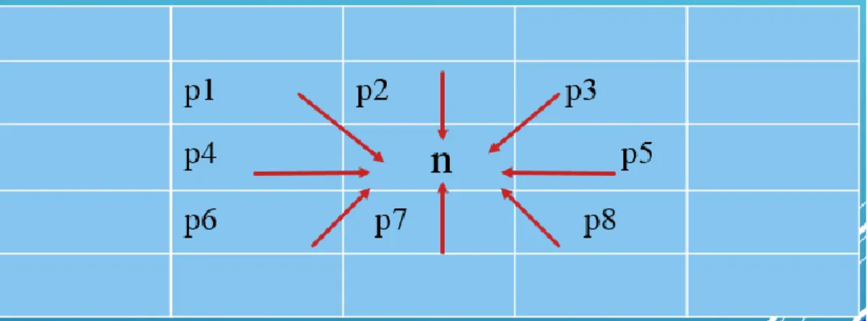
A* algorithm introducing parent node
Procedure of previous improved A* algorithm
Demonstration of improved A* algorithm
The following grid represents g(n) [actual cheapest cost to reach a cell from starting cell] for each adjacent cells of the current cell. The following grid represents h(n) [estimated cheapest cost to reach the goal from a cell n] for each adjacent cell in the current cell. So in the table above we can see that h(n) + g(n) is the same for all possible parents of the current cell.
But if we add value of h(p) with the previous value of h(n) + g(n), some cell will get more priority than others. Calculate the cost of principle (2,1) and add it to open list along with its cost. In step 1 all free (without obstacles) adjacent cell will be discovered in principle and they will be added in open list with their respective cost which will be calculated by formula f(n) = h(n) + h(p) + g (a).
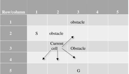
Start cell (2,1) is removed from the open list and added to the closed list. After step 1, there will be 4 information in the closed list and it will also be organized in ascending order of the cost of the cells. In step 2, the cell with the lowest cost from the open list is taken as the current cell, in this case cell (3,2).
All free (without obstacles) adjacent cells of the current cell will be discovered and they will be added to the open list with their respective costs which will be calculated by the formula f(n) = h(n) + h(p) + g(n ). The current cell (2,1) is removed from the open list and added to the closed list. After step 2, there will be 7 information in the closed list and it will also be organized in ascending order of the cost of the cells.
In step 3 the cell with the lowest cost from the open list will be taken as the current cell which in this case is cell (4,3). But meanwhile the goal cell (5,3) which is the cell adjacent to the current cell (4,3) will be found and the path from the starting cell to the goal cell will be saved. But when the heuristic value of the parent cell is added to the cost of a cell, there are still some opportunities to improve the performance of the algorithm.
Modification of improved A* algorithm
To increase the priority of the optimal cell when expanding the adjacent cell of a given cell, we will check which of those cells has the most chance to reach the goal. And we will add a certain value (let's call it V) to all cells adjacent to the current cell without the optimal one. And the V value will be added with all the adjacent cells without that optimal cell the whole cell.
So if this cell cannot reach the goal, all other cells will work as the normal A* algorithm. A cell that has a low heuristic value or in other words is close to the target, the value V because the adjacent cell will be lower than the cell that has a higher heuristic value. We take the row and column of the current cell and the row and column of the starting cell.
Then we calculate the ratio between the heuristic value of the current cell and the starting value of the current cell. And we multiply the ration by the product of the number of the row and the number of the column. So the value of V of staring cell will be (number of row * number of column).
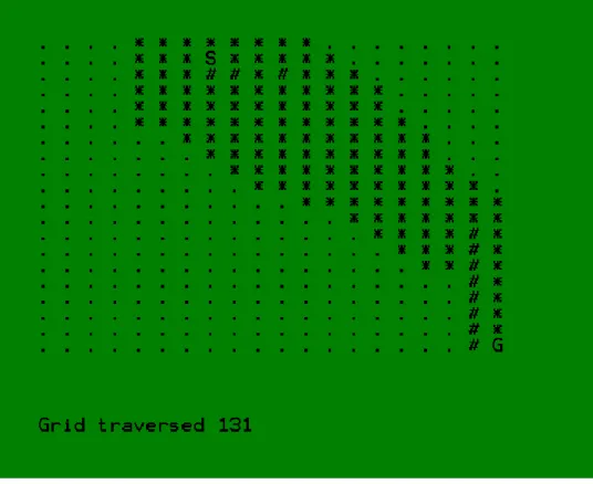
This method will expand less cell than previous improved algorithm because it will always try to check the optimal cells before the other cells. Following images demonstrate the expanded cell of previous improved algorithm and expanded cells of new modified algorithm for a specific environment. Principle is marked with S, target cell is marked with G, all traversed cell is marked with.
For this cell (20 * 20) with the start cell initialized at cell (1,8) and the goal cell starting at (20,20) the previous improved algorithm must traverse 222 grids before finding the goal cells. For this cell (20 * 20) with the start cell initialized at cell (1,8) and the goal cell starting at (20,20) the new modified algorithm must traverse 131 grids before finding the goal cells. From these two pictures it showed that the new modified version of the previous improved algorithm performs better.
Procedure of newly modified improved A* algorithm
The central idea of this newly modified algorithm is that it always tries to select the cell from the list that has more chances to reach the goal. Thus, the algorithm will always increase the priority of that cell type and give other cells their normal priority. So, if the optimal cell does not reach the target, the remaining cells will expand regularly.
And then the algorithm will try to find the optimal cells from the rest of the cells.
Search time
Path length
Number of traversed grid
Conclusions and Recommendations
Findings and Contribution
Recommendation for Future Work