In this thesis, an analytical approximate technique will be presented by combining the He's hornotopy perturbation technique and the extended form of the KBM method for the solution of certain types of fourth-order strongly nonlinear differential systems with small damping and cubic nonlinearity. The KBM method begins with the solution of a linear equation (sometimes called the generating solution of the linear equation), assuming that in the non-linear case, the amplitude and phase in the solution of the linear differential equation are time-dependent functions instead of of constants. This method imposes an additional condition on the first derivative of the assumed solution for determining the solution of a second-order equation.
Kruskal [23] extended the KB method to solve the fully nonlinear differential equation of the following form. It is observed that a basic differential equation (2.5) of the second order in the unknown x, reduces to two first order differential equations (2.14) and (2.15) in the unknowns a and o. They assumed the solution of the non-linear differential equation (2.5) of the form. 2.17) where Uk, (ki) are periodic functions of v with a period IT, and the quantities a and w are functions of time i and defined by the following first-order ordinary differential equations.
The solution of equation (2.4a) is based on recurrence relations and is given as a power series of the small parameter. Alan [29] has extended the KBM method to find solutions of nonlinear differential systems over damping, when one root of the auxiliary equation becomes much smaller than the other root. Alam [69] has also presented a modified and compact form of the unified KBM method for solving a nonlinear differential equation ;iih, n~ 2,3 of order.
79] investigated the solution of fourth-order critically damped oscillatory nonlinear systems when two of the eigenvalues are real and equal, and the other two are complex conjugate.
Introduction
An analytical approximation technique for solving a certain type of fourth-order strongly nonlinear oscillatory differential system with small damping. 9-1 1] presented an approximate technique for solving strongly nonlinear second-order oscillatory differential systems with damping effects combined with He homotopic perturbation and KBM methods. A more difficult and no less important case, strongly nonlinear fourth-order oscillatory differential systems with damping and cubic nonlinearity, remained almost untouched.
Therefore, in this chapter we are interested in developing a coupling analytical approximation technique, based on the He's homotopy perturbation and the KBM methods, to solve a certain type of fourth-order highly nonlinear oscillating differential systems with damping and cubic not to solve linearity. This method transforms a difficult problem under simplification into a simple problem which is easy to solve and understand and there is no complexity whatsoever in handling this method. The presented method has been successfully applied to solve a strongly nonlinear damped oscillating fourth-order differential system with an example.
The advantage of this method is that the first-order analytical approximation solutions s110w a good agreement with the corresponding numerical solutions.
The Proposed Method
Akbar el aL [76] presented the unified KBM method for solving a niche. states the nonlinear differential equation under some special conditions including internal resonance for a weakly nonlinear system. -1 1] have presented an approximate technique for solving strongly nonlinear second-order oscillatory differential systems with damping effects brushed with He homotopy blur and KBM methods. Many physical and engineering problems occur in nature which does not contain a small parameter, i.e. e., appear with strong damping and nonlinearity.
3.2) r Differentiating equation (3.2) four times with respect to time I, and then substituting the derivatives PI,Y, 1, ± together with x and the values of p and q in equation (3.1.) and simplifying them , we get . Equation (3.4) can be rewritten as. Here U) is a constant for the damped nonlinear oscillator and known as frequency in the literature and A. But, for damped nonlinear oscillatory differential systems, t is a time-dependent function and it varies slowly with time t.
To solve this situation, we can use the extended form of the KBM method [2-3] of Mitropolski [4]. According to this method, we choose the solution of equation (3.5) (for a single oscillation mode) in the following form. Now, if we differentiate equation (3.7) four times with respect to time / and apply equation (3.8) and then take terms up to 0(s), we get
Equation (3.18) represents the first-order approximate analytical solution of equation (3.1) with the proposed coupling technique. Thus, the determination of approximate analytical solutions of the first order of equation (3.1) is completed by the proposed method.
Example
3.32) Now, putting equation (3.32) into equation (3.13) and taking the terms for 0(e), we get
Results and Discussion
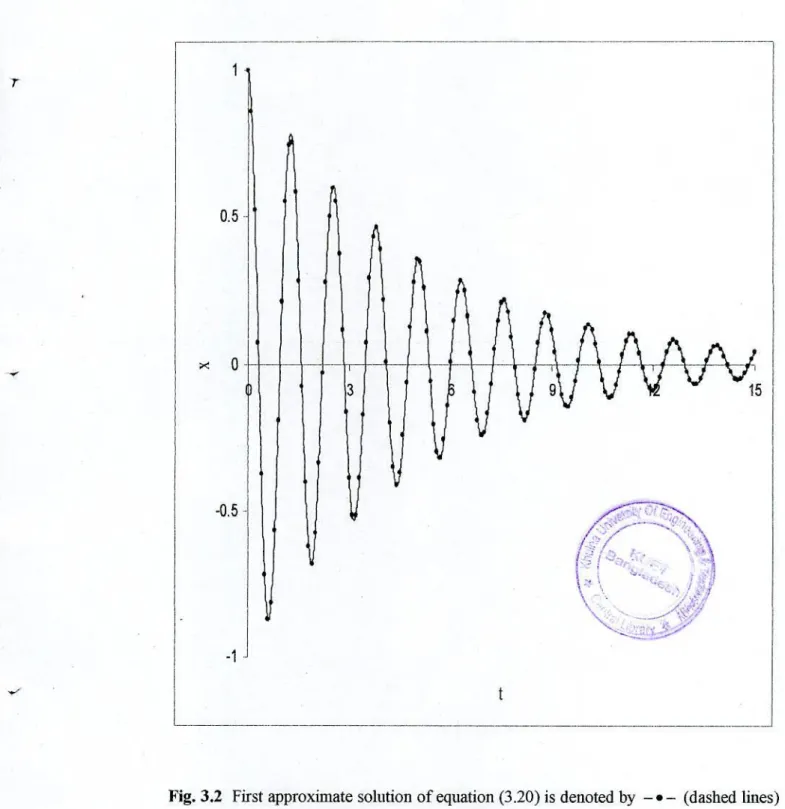
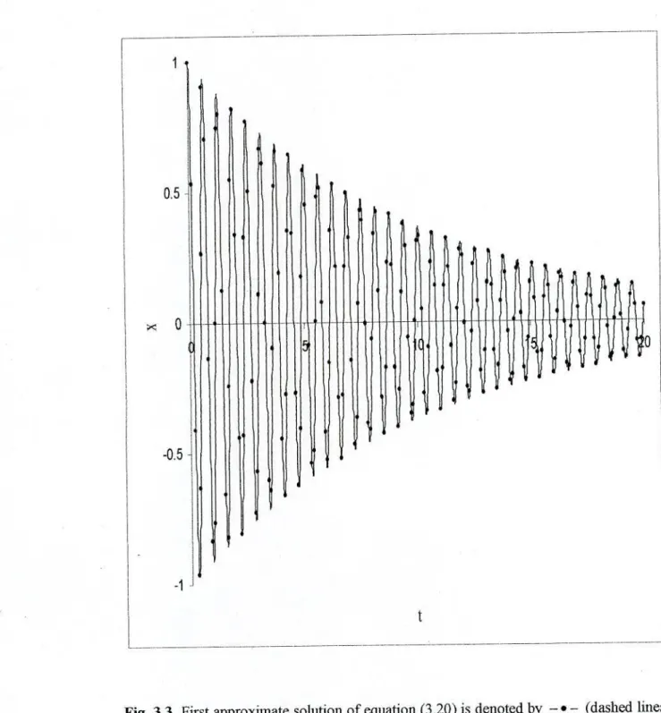
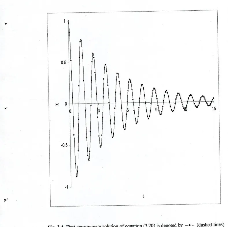
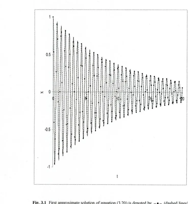
In this chapter, a new coupling analytical approximate technique has been presented to obtain first-order analytical approximate solutions for a certain type of fourth-order strongly nonlinear oscillating differential systems with damping, and the method is successfully implemented to illustrate the effectiveness and convenience of proposed method. The first-order analytical approximate solutions of equation (3.20) are calculated using equation (3.37) using equations and equation (3.36), and the corresponding numerical solutions are obtained by the well-known fourth-order Runge-Kutta method. Furthermore, the presented method is simple and the advantage of this method is that the first-order approximate solutions show good agreement (see also Figs. 3.1-3.4) with the corresponding numerical solutions for several damping effects.
The approximations obtained by the proposed method are not only valid for strong nonlinear oscillatory differential systems, but also for weak one with small damping effects. 3.1-3.2 are provided to compare the solutions obtained by the proposed method with the corresponding numerical solutions with small damping for strongly nonlinear oscillatory differential systems. 3.3-3.4 are cited to compare the solutions obtained by the proposed method with the corresponding numerical solutions for weakly nonlinear oscillatory differential systems with small damping effects.
3.1-3.4 it can be seen that the approximate analytical solutions obtained for both strongly and weakly nonlinear differential systems show good agreement with those solutions obtained by the fourth-order Runge-Kutta method.
Introduction
The Method
It is assumed that the function f(°) can be expanded into power series (Taylor's series) of the form (see also [31 for details). 721 have imposed the condition that Ut does not contain the fundamental terms (the solution presented in equation (4.2) is called generating solution and its terms are called fundamental terms) of f(s). These relations are important because under these relations the coefficients in the solutions of A1, A3 and A4 do not become large.
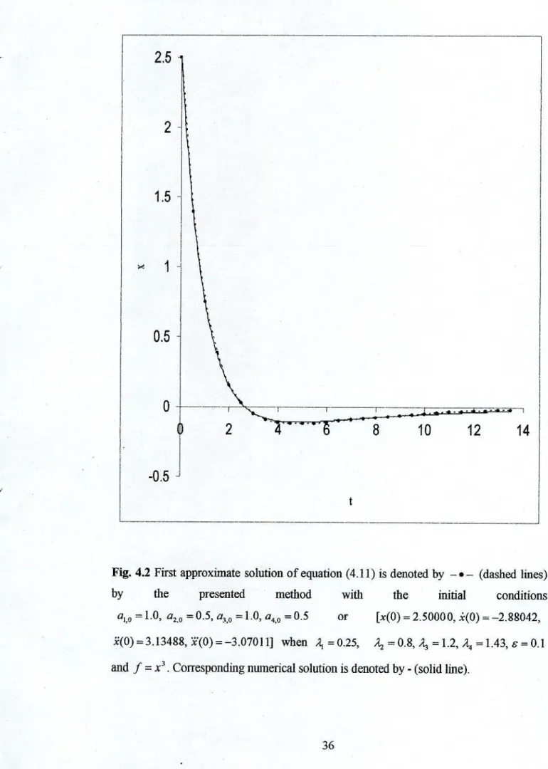
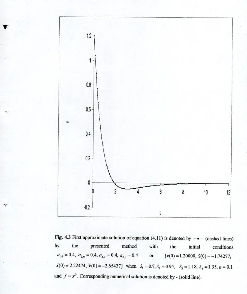
So they are slowly varying functions of time i, which means that they are almost constant and by integration we get the values of a, (I. As an example of the above method, we consider the following nonlinear differential equation of the fourth order. Under these imposed conditions and by equating similar terms on both sides of the equation (4.13) we get.
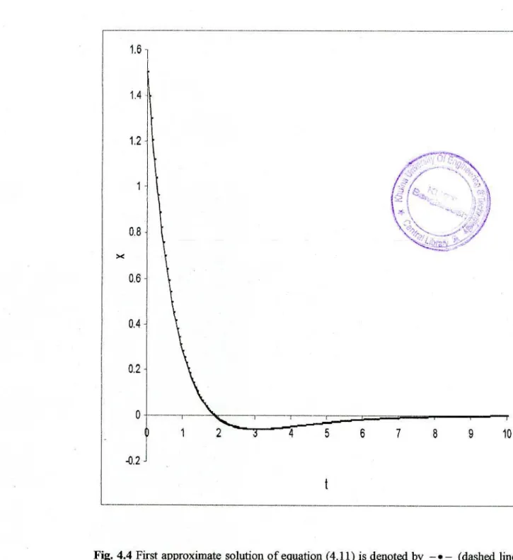
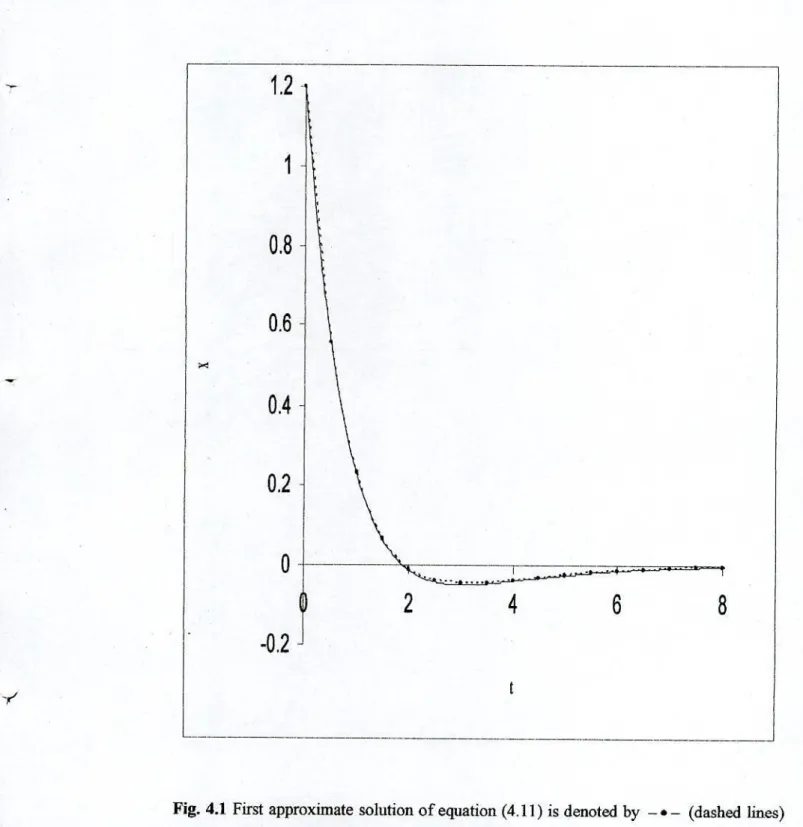
To test the accuracy of the estimated analytical solutions obtained by the presented technique, they were compared with the numerical solutions. The corresponding numerical solution of equation (4.11) is calculated using the fourth-order Runge-Kufta method. The approximate analytical solutions and numerical solutions are plotted in the figures.
CHAPTER 5
Vitro and Cabak G., Effects of internal resonance in two-degree-of-freedom impulsive forced nonlinear systems, Jut.