Since view buffer is used to store view list and is used to refresh it is also called refresh buffer. The continuous low speed electrons from the flood gun pass through the control grid and are attracted to the positively charged region of the storage grid.
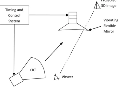
Three dimensional viewing devices
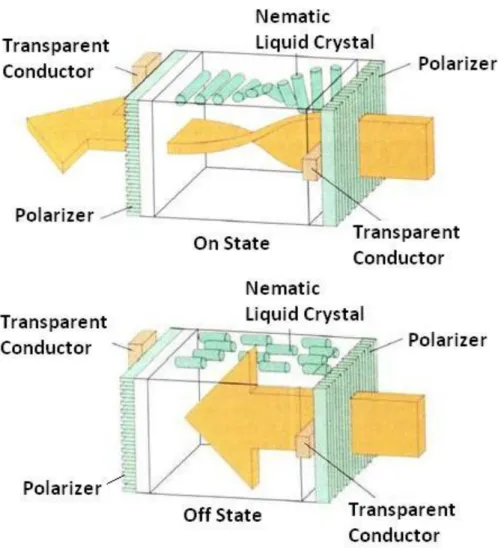
Transistor causes crystal to change their state rapidly and also to control the degree to which the state is changed.
Stereoscopic and virtual-reality systems Stereoscopic system
Virtual-reality
A headset containing an optical system to create stereoscopic views is typically used in conjunction with interactive input devices to locate and manipulate objects in a scene. Virtual reality can also be created using stereoscopic glass and a video monitor instead of a headset.
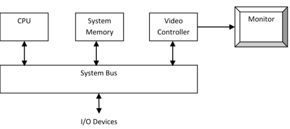
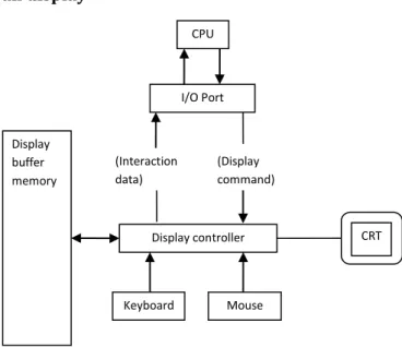
Raster graphics systems Simple raster graphics system
Sensor in the headset keeps track of the viewer's position so that the front and back of objects can be seen as the viewer "walks through" and interacts with the screen.
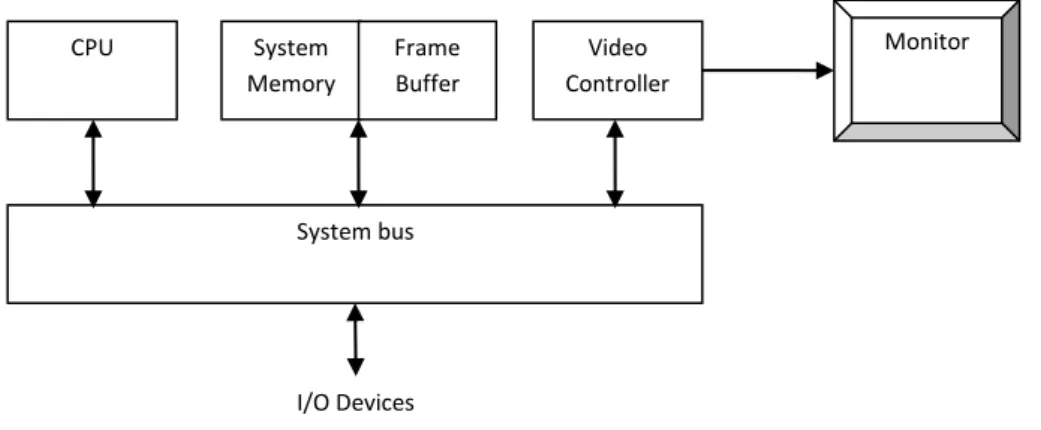
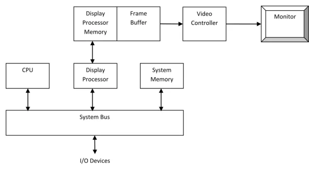
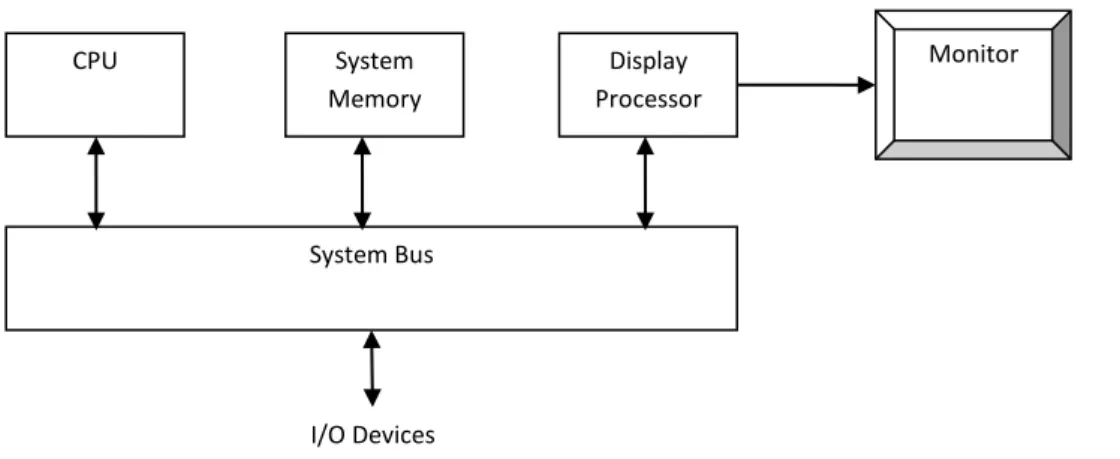
Raster graphics system with a fixed portion of the system memory reserved for the frame buffer
The value stored in framebuffer for this pixel is retrieved and used to set the intensity of the CRT beam. The main job of the display processor is to digitize a picture definition given into a set of pixel intensity values to store in frame buffer.

Random- scan system
Mouse
Trackball and Spaceball
Spaceball strain gauges measure the amount of pressure applied to the spaceball to provide data on spatial positioning and orientation as the ball is pushed or pulled in different directions. Spatial balls are used in 3D positioning and selection operations in virtual reality system, modeling, animation, CAD and other applications.
Joysticks
Data glove
Digitizer
Touch Panels
When we touch at a certain point, the line of the light path is broken and the coordinate values are measured according to this broken line. When the two plates touch, it creates a voltage drop across the resistive plate, which is converted into the coordinate values of the selected position.
Light pens
The optical touch panel uses an infrared LED line along one vertical and one horizontal edge. These reflected waves arrive back at the transmitter position and the time difference between sending and receiving is measured and converted into coordinate values.
Voice systems
Another system can be adapted for touch input by placing a transparent touch-sensing mechanism on the screen. The general software package provides an extensive set of graphics functions that can be used in a high-level programming language such as C or FORTRAN.
Coordinate representations
Special purpose application packages are tailor-made for a specific application, which implements the required facility and provides an interface so that the user does not have to worry about how it will work (programming).
Software Standard
Points and Lines
Line Drawing Algorithms
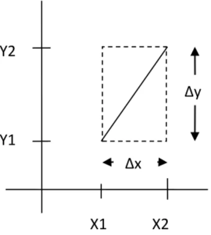
DDA Algorithm
Since 𝑚 can be any real number between 0 and 1, the calculated 𝑦 values must be rounded to the nearest whole number. Above, both comparisons are based on the assumption that lines should be processed from left endpoint to right endpoint.
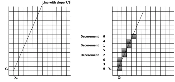
Bresenham’s Line Algorithm
This recursive calculation of the decision parameters is performed at each position of the integer 𝑥 starting at the endpoint of the left coordinate of the line. Bresenham's algorithm is generalized to lines of arbitrary slope by considering the symmetry between different octants and quadrants of the 𝑥𝑦 plane.
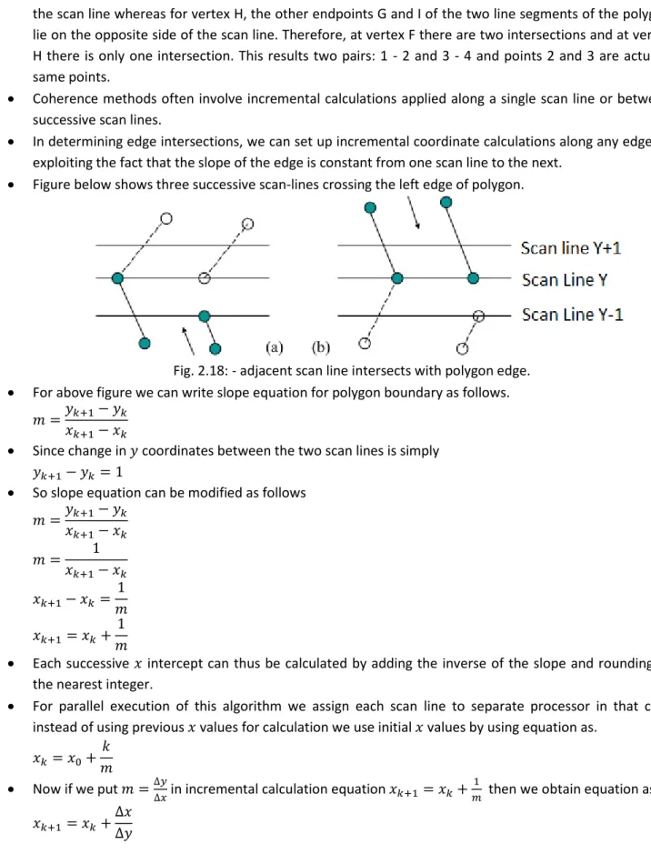
Parallel Execution of Line Algorithms
The extension of the parallel Bresenham algorithm to a line with slope greater than 1 is obtained by dividing the line in the 𝑦 direction and computing initial 𝑥 values for the positions. This approach can be adapted for line display by assigning one processor to each of the pixels within the boundary of the bounding rectangle and calculating pixel distance from the line path.
Circle
Each processor calculates line intersection with horizontal row or vertical column pixels assigned to that processor. If vertical column is assigned to processor then 𝑥 is fixed and it will calculate 𝑦 and similarly horizontal row is assigned to processor then 𝑦 is fixed and 𝑥 will be calculated.
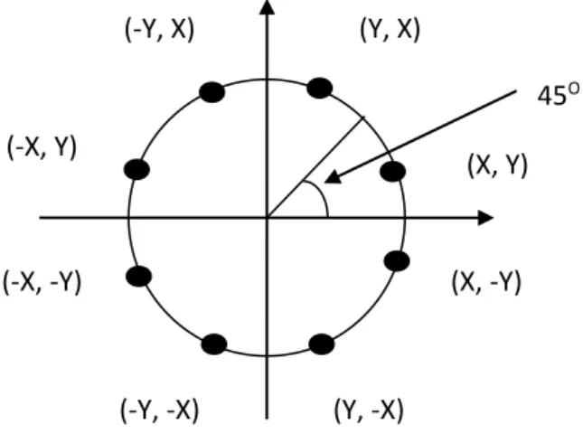
Properties of Circle
Taking advantage of this property of circle symmetry, we can generate the entire pixel position on the boundary of the circle by computing just one sector from 𝑥 = 0 to 𝑥 = 𝑦. Determining the position of the pixel along the circumference of the circle using either of the two equations presented above still required large calculations.
Midpoint Circle Algorithm
The initial decision parameter is obtained by evaluating the circle function at the starting position (𝑥0, 𝑦0) = (0, 𝑟) as follows. Enter radius 𝑟 and circle center (𝑥𝑐, 𝑦𝑐) to obtain the first point on the circumference of a circle centered on the origin axis.
Ellipse
Properties of Ellipse
The equation of the ellipse shown in Figure 2.12 can be written in terms of the coordinates and parameters of the ellipse center 𝑟𝑥 and 𝑟𝑦 axis. So we need to calculate the cutoff point for one quadrant and then the other three quadrant points can be obtained by symmetry as shown in the figure below.
Midpoint Ellipse Algorithm
Suppose we are in (𝑥𝑘 , 𝑦𝑘) position and we determine the next position along the ellipse path by evaluating decision parameter at the midpoint between two candidate pixels. If 𝑝2𝑘 > 0, the center point is outside the ellipse boundary and we select the pixel at 𝑥𝑘.
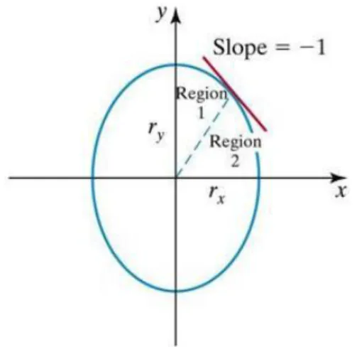
Filled-Area Primitives
In the above case we take the unit step in the positive 𝑦 direction to the last selected point in region 1. Calculate the initial value of the decision parameter in region 2 using the last point (𝑥0, 𝑦0) calculated in region 1 as .
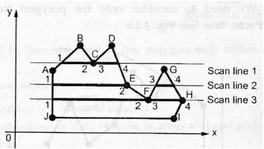
Scan-Line Polygon Fill Algorithm
Conformance methods often involve incremental calculations applied along a single scan line or between successive scan lines. Each table entry for a particular scan line contains the maximum 𝑦 values for those edges, the 𝑥 intercept value for the edge, and the inverse slope of the edge.
Inside-Outside Tests
We then process the scan line from bottom to top for the entire polygon and produce an active edge list for each scan line that crosses the polygon boundaries. The active edge list for a scan line contains all edges intersected by that line, with iterative coherence computation used to obtain the edge intersections.
Odd Even Rule
Nonzero Winding Number Rule
Comparison between Odd Even Rule and Nonzero Winding Rule
Scan-Line Fill of Curved Boundary Areas
Boundary Fill Algorithm/ Edge Fill Algorithm
This method fills horizontal pixel stretches across scan lines, instead of continuing to 4 connected or 8 connected neighboring points. An example of how pixel regions can be filled using this approach is illustrated for the 4-connected fill region in Figure below.
Flood-Fill Algorithm
Character Generation
Bitmap Font/ Bitmapped Font
Outline Font
The small series of line segments are drawn like a pen stroke to form a character as shown in figure. Here it is necessary to decide which line segments are required for each character and then draw that line to display character.
Starbust Method
Line Attributes
Line Type
Line Width
If we change the width of the line, we can also change the line ending. The three types of ends are illustrated below. Similarly, we generate connections from two lines with changed width, as shown in the image below, illustrating all three types of connections.
Line Color
In raster images, we generate thick lines by plotting above and below the line path pixel at slope |𝑚| < 1 and by plotting the left and right pixels of the line path at slope |𝑚| > 1, as shown in the image below.
Pen and Brush Options
Color and Greyscale Levels
24 bit color values are stored in the lookup table and in the frame buffer we store only an 8 bit index, which gives the index of the required color stored in the lookup table. When we display an image on the output screen using this technique, we look in the frame buffer where the index of the color is stored and take the 24-bit color value from the lookup table that corresponds to the index value of the frame buffer and display that color on a particular pixel.
Greyscale
Area-Fill Attributes
Fill Styles
Pattern Fill
Soft fill is a custom border fill and filling algorithm where we fill a color layer on the background color so that we can get the combination of both colors. It is used to recolor or repaint so that we can obtain a multi-color layer and get a new color combination.
Character Attributes
One use of this algorithm is to soften the fill at the boundary so that the blur effect will reduce the aliasing effect. If we use more than two colors, say three at the time, the equation becomes as follows:
Text Attributes
Text is then displayed so that the orientation of characters from baseline to mainline is in the direction of the up vector. Where the text precision parameter tpr is assigned one of the values: string, char or dash.
Marker Attributes
Where the text path parameter tp can be assigned a value: right, left, up, or down. The highest quality text is produced when the parameter is set to the pod value.
Transformation
Basic Transformation
Translation
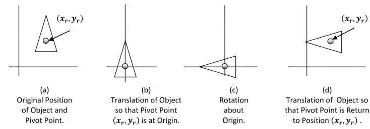
Rotation
These equations differ from rotation about the origin and the matrix representation is also different. Rotation is also a rigid body transformation, so we need to rotate every point of the object.
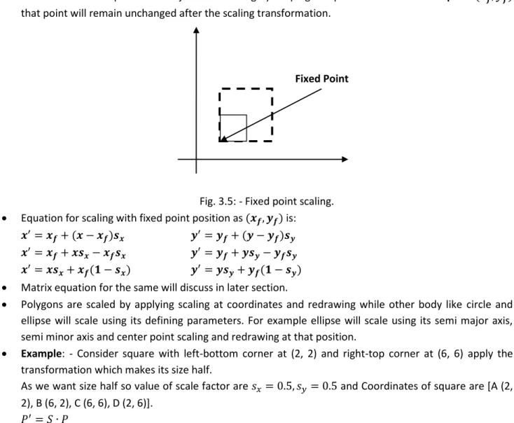
Scaling
The matrix equation can be obtained by a simple method that we will discuss later in this chapter. Values less than 1 decrease the size, while values greater than 1 increase the size of the object, and the object remains unchanged when the values of both factors are 1.
Matrix Representation and homogeneous coordinates
Composite Transformation
Move the object so that the pivot point returns to its original position (ie the inverse of step 1). Move the object so that the fixed point returns to its original position (ie, the inverse of step 1).
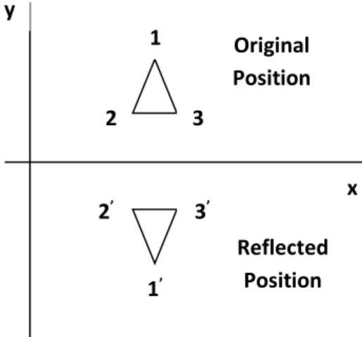
Other Transformation
The mirror image for a two-dimensional reflection is generated relative to a reflection axis by rotating the object 180o about the reflection axis. This transformation keeps x-values the same, but inverts (changes the sign) y-values of coordinate positions.
The Viewing Pipeline
We then map the viewing coordinate to the normalized viewing coordinate, obtaining values between 0 and 1. Finally, we convert the normalized view coordinate to device coordinate using device drivers that provide device specification.
Viewing Coordinate Reference Frame
By resizing the window and viewport, we can achieve zoom in and zoom out effect as per requirement. Viewports are usually defined with the unit square so that graphics package is more device independent, which we call as normalized view coordinate.
Window-To-Viewport Coordinate Transformation
Clipping Operations
Point Clipping
Line Clipping
And for the partial inner line, we need to calculate the intersection with the window boundary and find out which part is inside the clipping boundary and which part is excluded.
Cohen-Sutherland Line Clipping
Region and Region Code
Algorithm
Draw line segment that is completely inside and eliminate other line segment that is completely outside.
Intersection points calculation with clipping window boundary
Liang-Barsky Line Clipping
Advantages
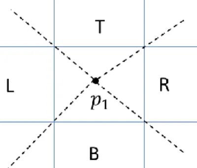
Nicholl-Lee-Nicholl Line Clipping
For example, p1 is in the edge region and to check whether p2 is in the region LT we use the following equation. For the left and right bounds we compare 𝑥-coordinates and for the upper and lower bounds we compare 𝑦-coordinates.
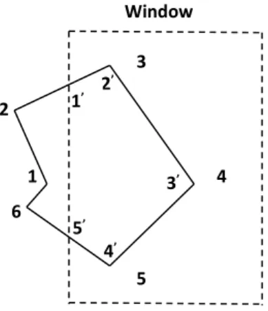
Polygon Clipping
As shown in example 1: if both points are inside the window, we only add the second point to the output list. From v3 to v4 we calculate the intersection and add to the output list and follow the window border.
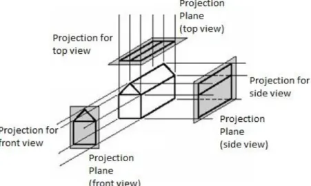
Three Dimensional Display Methods Parallel Projection
Perspective projection
Depth cueing
A simple method for this is depth cues, where you assign higher intensity to closer objects and lower intensity to distant objects.
Visible line and surface Identification
Surface Rendering
Exploded and Cutaway views
Three dimensional stereoscopic views
To achieve this, we first need to get two views of object generated from the viewing direction corresponding to each eye. One way to produce stereoscopic effect is to display each of the two views rasterized on alternate refresh cycles.
Polygon Surfaces
We can summarize the two views as computer-generated scenes with different viewing positions, or we can use a stereo camera pair to photograph an object or scene. When we simultaneously see both the left view with the left eye and the right view with the right eye, two views are merged to create an image that appears to have depth.
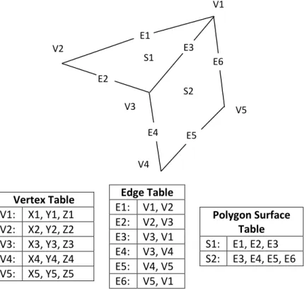
Polygon Tables
Edge table stores each edge with the two endpoint vertex pointers back to the vertex table. Polygon table stores each surface of polygon with edge marker for each edge of the surface.
Plane Equations
Polygon Meshes
Spline Representations
Interpolation and approximation splines
Parametric continuity condition
Geometric continuity condition
Cubic Spline Interpolation Methods
Natural Cubic Splines
Hermit Interpolation
It is adjusted locally because each curve section depends only on the endpoints. Where 𝐻𝑘(u) for k are called blend functions because they combine the boundary constraint values for the curve section.
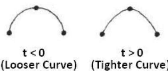
Cardinal Splines
Hermit curves are used in digitizing applications where we enter the approximate curve slope means DPk. 12 Where parameter t is called tension parameter as it controls how loosely or tightly the cardinal note fits the control points.
Kochanek-Bartels spline
Bezier Curves and Surfaces
Bezier Curves
The efficient method for determining coordinate positions along a Bezier curve can be established using recursive computation.
Properties of Bezier curves
Design Technique Using Bezier Curves
4.22: -A Bezier curve can be made to pass closer to a given coordinate position by assigning more control points at that position. Similarly for second-order continuity the third control point of the second curve in terms of position of the last three control points of the first curve section as.
Cubic Bezier Curves
The continuity of C2 can be unnecessarily restrictive, especially with a cubic curve we left only one control point to adjust the shape of the curve. Another mixing function affects the shape of the curve at intermediate values of the u parameter.
Bezier Surfaces
Spline Curves and Surfaces
The degree of the B-spline polynomial can be set independently of the number of control points (with a certain limit).
Spline Curves
Properties of B-Spline Curves
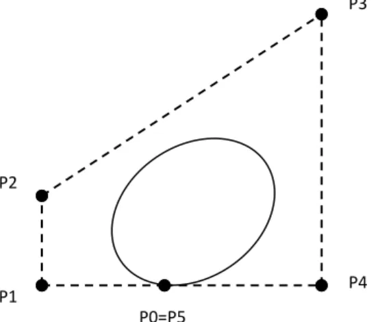
Uniform Periodic B-Spline
Cubic Periodic B-Spline
We can obtain cubic B-Spline mixture function for parametric range from 0 to 1 by converting matrix representation to polynomial form for t = 1 we have.
Open Uniform B-Splines
Non Uniform B-Spline
Spline Surfaces
3D Translation
Axis Rotation
- Axis Rotation
The x-axis transformation equation is obtained from the z-axis rotation equation by substituting cyclic as shown here.
Axis Rotation
General 3D Rotations when rotation axis is parallel to one of the standard axis
General 3D Rotations when rotation axis is inclined in arbitrary direction
To do this, we repeat the above procedure between 'u' and 'uz' to find the matrix for rotation around the Y-axis. As we know, we align the rotation axis with the Z axis, so now a matrix for rotation around the z axis.
Coordinate Axes Scaling
Now by combining both rotation, we can coincide axis of rotation with Z axis 3) Perform the specified rotation around that coordinate axis. We can apply uniform as well as non-uniform scaling by choosing the right scaling factor.
Fixed Point Scaling
Other Transformations Reflections
Shears
Viewing Pipeline
Viewing Co-ordinates
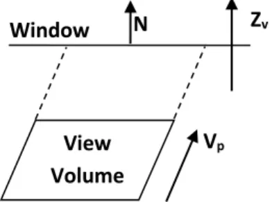
Specifying the view plan
Next we select positive direction for the view Zv axis and the orientation of the view plane by specifying the view plane normal vector N . Finally, we choose the upward direction for the view by specifying a vector V called the view-up vector.
Transformation from world to viewing coordinates
The viewing reference point is often chosen close to or on the surface of the same object scene. By fixing the facial reference point and changing the direction of the normal vector N, we get different views of the same object. This is illustrated in the figure below.
Projections
In the general case, N is in arbitrary direction, then we can align it with the coordinate axes of words with rotation sequence 𝑅𝑧 ∙ 𝑅𝑦 ∙ 𝑅𝑥. This transformation is applied to the object's coordinates to transfer them to the viewing reference frame.
Parallel Projections
A parallel projection can be defined by a projection vector, which defines the direction for the projection lines. When the two projection lines are perpendicular to the plane of view, we have a perpendicular parallel projection.
Perspective Projection
We control the number of principal vanishing points (one, two, or three) with the orientation of the projection plane, and perspective projections are therefore classified as one-, two-, or three-point projections. The number of principal vanishing points in a projection is determined by the number of principal axes that intersect the plane of view.
View Volumes and General Projection Transformations
General Parallel-Projection Transformation
As shown in the figure, the parallel projection is defined by the projection vector from the projection reference point to the viewing window. Thus, we have a general parallel projection matrix in terms of the elements of the projection vector as
General Perspective-Projection Transformations
Classification of Visible-Surface Detection Algorithms
Back-Face Detection
Depth Buffer Method/ Z Buffer Method
If the calculated depth value is greater than the value stored in the depth buffer, it will be replaced by new calculated values and the intensity of that point will be stored in the refresh buffer at the (x,y) position. To do this, if we move from top to bottom along the polygon boundary, we get x'=x-1/m and y'=y-1, so the z value is obtained as follows.
Light source
A nearby source such as the long fluorescent light is more accurately modeled than a diffuse light source. The amount of reflected and absorbed light depends on the property of the object surface.
Basic Illumination Models/ Shading Model/ Lighting Model
In this case, the lighting effects cannot be approximated with a point source, because the area of the source is not small compared to the size of the object. When light falls on the surface, some of the light is reflected and some of the light is absorbed.
Ambient Light
This light source model is a reasonable approximation for a source whose size is small compared to the size of the object or may be far enough away for us to see it as a point source.
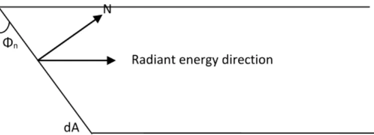
Diffuse Reflection
Although there is equal light distribution in all directions from a perfect reflector, the brightness of a surface depends on the orientation of the surface with respect to the light source. 6.8: angle of incidence 𝜃 between the direction vector L of the unit's light source and the unit's surface normal N.
Specular Reflection and the Phong Model
Here, the ambient reflection coefficient 𝐾𝑎 is used in many graphics packages, so here we use 𝐾𝑎 instead of 𝐾𝑑. A somewhat simplified phong model is to calculate between the half-path vectors H and use the product of H and N instead of V and R.
Combined Diffuse and Specular Reflections With Multiple Light Sources
Properties of Light
Intensity is the radiant energy emitted per unit time, per unit solid angle and per unit projected area of the source. The purity or saturation of the light describes how washed out or how "pure" the color of the light appears.
XYZ Color Model
This frequency reflected back determines the color we see and this frequency is called dominant frequency (hue) and corresponding reflected wavelength is called dominant wavelength. Typical color models used to describe combinations of light in terms of dominant frequency use three colors to achieve a reasonably wide range of colors, called the color gamut of that model.
RGB Color Model
Two or three colors used to get other colors in the range are called primary colors. So, by combining these three colors, we can get a wide range of colors, this concept is used in the RGB color model.
YIQ Color Model
Since it is bounded between unit cube, its values are very much between 0 and 1 and it is represented as triplet (R,G,B).
CMY Color Model