IMPACT OF FORECAST MODELING ON COST
PERFORMANCE
TAN KAH EE B050710002
UNIVERSITI TEKNIKAL MALAYSIA MELAKA
IMPACT OF FORECAST MODELING ON COST PERFORMANCE
This report submitted in accordance with requirement of the Universiti Teknikal Malaysia Melaka (UTeM) for the Bachelor Degree of Manufacturing Engineering
(Manufacturing Management)
by
TAN KAH EE B050710002
UNIVERSITI TEKNIKAL MALAYSIA MELAKA
BORANG PENGESAHAN STATUS LAPORAN PROJEK SARJANA MUDA
TAJUK: Impact of Forecast Modeling on Cost Performance
SESI PENGAJIAN: 20010/11 Semester 2
Saya TAN KAH EE
mengaku membenarkan Laporan PSM ini disimpan di Perpustakaan Universiti Teknikal Malaysia Melaka (UTeM) dengan syarat-syarat kegunaan seperti berikut:
1. Laporan PSM adalah hak milik Universiti Teknikal Malaysia Melaka dan penulis.
2. Perpustakaan Universiti Teknikal Malaysia Melaka dibenarkan membuat salinan untuk tujuan pengajian sahaja dengan izin penulis.
DECLARATION
I hereby, declared this report entitled “Impact of forecast modeling on cost performance.” is the results of my own research except as cited in references.
Signature : ………
Author’s Name : Tan Kah Ee
APPROVAL
This report is submitted to Faculty of Manufacturing Engineering of UTeM as a partial fulfillment of the requirements for the degree of Bachelor of Manufacturing Engineering (Manufacturing Management). The member of the supervisory committee is as follow:
……… Supervisor
i
ABSTRAK
Secara umumya, kebanyakan pentadbiran dan pengurusan industri cenderung untuk mencari dan melaksanakan pendekatan sederhana untuk masalah-masalah operasi yang dihadapi dalam aktiviti harian. Dalam projek ini, penulis merujuk kepada pendekatan sederhana yang difahami oleh pengurus-pengurus. Para pengurus tidak akan merujuk kepada pendekatan yang mereka kurang fahami bagi mengelakkan risiko yang akan
ditanggung akibat membuat keputusan yang salah. “Exponential Smoothing” dan
“Moving Average” merupakan kaedah ramalan yang paling umum bagi meramal
permintaan pelangan seperti mana dilapor dalam “Literature Review”. Selain itu, penulis
ii
ABSTRACT
iii
ACKNOWLEDGEMENT
First and foremost, the author would like to express the deepest gratitude to the Final Year Project supervisor, En. Nor Akramin b. Mohamad for his supervision and encouragement along the project duration. His advice and encouragement plays an important role to the project completion.
The author would like to thanks also persons that provided support and assistance to the project such as fellow course mates and lecturers. It was deeply appreciated regards to their helpful gesture.
iv
DEDICATION
v
1.3 Research Objectives 6
1.4 Research Scope 6
1.5 Organization of Report 7
2. LITERATURE REVIEW 9
2.1 Forecasting 9
2.1.1 Steps in the forecasting 11
2.1.2 Advantages of forecasting 11
2.1.3 Forecast techniques 12
2.1.4 Forecast Error 13
2.2 Inventory Control System 15
3. METHODOLOGY 20
vi
3.1.1 Define Problem, Objective, and Scope 20
3.1.2 Literature Review 21
3.1.3 Model Development 21
3.1.4 Model Testing 22
3.1.5 Result Analysis 22
3.1.6 Report Findings 23
3.2 Project Methodology 23
3.3 Solution Methodology 24
3.4 Gantt Chart 25
4. THE CONCEPT OF FORECASTING MODELS AND INVENTORY
MODELS 26
4.1 Forecasting models 26
4.1.1 The concept of Exponential Smoothing 26
4.1.1.1 Simple Exponential Smoothing 26
4.1.1.2 Double Exponential Smoothing 27
4.1.1.3 Smoothing Constant 31
4.1.2 The concept of Moving Average 31
4.1.2.1 Simple Moving Average 32
4.1.2.2 Weighted Moving Average 33
4.1.3 Forecasting Error 35
4.1.3.1 Mean Absolute Deviation (MAD) 35
4.1.3.2 Mean Squared Error (MSE) 37
4.1.3.3 Mean Absolute Percent Error (MAPE) 39
4.2 Inventory Modeling 40
4.2.1 Single-Period Model 40
4.2.2 Fixed-Period System 42
4.2.3 Basic Economic Order Quantity (EOQ) 44
5. PROBLEM DESCRIPTION 46
vii
5.1.1 Inventory Control of Central Depot 48
5.2 Model Formulation 51
5.2.1 Description of the proposed model 51
5.2.2 Description of the Project Model 52
5.2.2.1 Demand Forecasting Model 52
5.2.2.2 Order Point 54
5.2.2.3 Order-up-to level 54
5.2.2.4 Order Quantity 54
5.2.2.5 Number of Pallet 55
5.2.2.6 Coordinated Replenishment Policy (CRP) 55
5.3 Model Contribution and Modification 55
5.3.1 Assumptions made 56
5.3.2 Simplifications 58
5.4 Design of Experiment 58
5.4.1 Input Validity 59
5.4.2 Forecasting Models Validity 61
5.4.3 Designed Scenario 61
6.1.1.1 Phase 1: Input parameter column checking 64
6.1.1.2 Phase 2: Model components checking 65
6.1.1.3 Phase 3: Function testing 65
6.1.1.4 Phase 4: Model flow testing 67
6.1.1.5 Phase 5: Model verifying 67
viii
6.1.2.1 Phase 1: Input parameter column checking 68
6.1.2.2 Phase 2: Model components checking 68
6.1.2.3 Phase 3: Function testing 69
6.1.2.4 Phase 4: Model flow testing 69
6.1.2.5 Phase 5: Model verifying 69
6.2 Model Validation 70
6.2.1 Manual Calculation 72
6.2.1.1 Inventory control system 72
6.2.1.2 Cost model 75
6.2.2 Result from MS Excel Model 76
6.2.2.1 Inventory control model 76
6.2.2.2 Cost model 76
6.3 Results and findings 78
7. CONCLUSION 89
REFERENCES 91
APPENDICES
A Stationary demand
B Trend demand
C(I) Scenario A: Double Exponential Smoothing with trend demand (Forecast
result)
C(II) Scenario A: Double Exponential Smoothing with trend demand (Inventory
result)
C(III) Scenario A: Double Exponential Smoothing with trend demand (Total cost result)
D(I) Scenario B: Moving Average with trend demand (Forecast result)
D(II) Scenario B: Moving Average with trend demand (Inventory result)
ix
D(IV) Scenario B: Simple Exponential Smoothing with trend demand (Forecast result)
D(V) Scenario B: Simple Exponential Smoothing with trend demand (Inventory
result)
D(VI) Scenario B: Simple Exponential Smoothing with trend demand (Total cost result)
E(I) Scenario C: Moving Average with stationary demand (Forecast result)
E(II) Scenario C: Moving Average with stationary demand (Inventory result)
E(III) Scenario C: Moving Average with stationary demand (Total cost result) E(IV) Scenario C: Simple Exponential Smoothing with stationary demand (Forecast
result)
E(V) Scenario C: Simple Exponential Smoothing with stationary demand (Inventory
result)
E(VI) Scenario C: Simple Exponential Smoothing with stationary demand (Total cost result)
F(I) Scenario D: Double Exponential Smoothing with stationary demand (Forecast
result)
F(II) Scenario D: Double Exponential Smoothing with stationary demand
(Inventory result)
F(III) Scenario D: Double Exponential Smoothing with stationary demand (Total cost result)
x
LIST OF TABLES
4.1 Table of Exponential Smoothing with Trend Adjustment 26
4.2 A review of past sales 27
4.3 Forecast with ∝= .2 and = .4 28
4.4 Smoothing Constant with weighted period 29
4.5 Demand for shopping carts for the last five periods 31
5.1 List of variable information based on products 57
5.2 Stationary demand before adjustment 59
5.3 Mean Value if trend demand 60
5.4 Stationary demand after adjustment 60
5.5 Trend demand 60
6.6 Output performance measure of costs 78
6.7 Correlation coefficient between cost 78
6.8 Simulation output for number of truckload 79
xi
6.10 Correlation analysis of cost performance, truckload utilization, and number of
truckload 80
6.11 Simulation output of mean inventory control parameter for each product 81
6.12 Mean of mean analysis for inventory control parameter 81
6.13 Simulation outputs for forecast performance measure of Product A 84
6.14 Simulation outputs for forecast performance measure of Product B 85
6.15 Simulation outputs for forecast performance measure of Product C 85
6.16 Mean of forecast performance measures 85
6.17 Summary of simulation outputs 87
xii
5.3 Inventory Model Simulation Flow Chart 50
6.1 Procedure flow for Model Verification 64
6.2 Process flow for Validation 71
6.5b Total cost vs. inventory on-hand updated 82
6.5c Total cost vs. order up-to-level 82
6.5d Total cost vs. order quantity 83
6.6 Forecast error base analysis 86
xiii
LIST OF ABBREVIATIONS
CRP - Coordinated Replenishment Policy
EOQ - Economic Order Quantity
MAD - Mean Absolute Deviation
MAPE - Mean Absolute Percent Error
MROs - Maintenance/ Repair/ Operating
MSE - Mean Square Error
ROP - Reorder Point
WIP - Work In Progress
SES - Simple Exponential Smoothing
DES - Double Exponential Smoothing
1
CHAPTER 1
INTRODUCTION
This project investigate the impact of forecasting modeling on transportation and inventory carrying cost of an environment that consists of inventory management of a central depot. In this chapter, the following topics will be addressed: overview is first introduced, followed by research problem, objectives, and scope of project.
1.1Overview
2
1.1.1 Forecasting
Forecasting is an art and science of predicting future events (Heizer and Render, 2010). In an overview of forecasting, there is classified into two methods: quantitative forecasting method and qualitative forecasting method. Qualitative forecast method is based on educated opinion of appropriate person whereas quantitative forecast method is more to time series analysis such as historical data analysis and component of time series demand. Some examples of qualitative forecast method include Delphi Method, market research, product life-cycle analogy, and expert judgment (“Forecast”, 1997). For quantitative forecast method, which is the interested part in this project, there are two parts of concerns. Part 1 is the time-series forecasting modeling which is forecast the new demand based on historical data such as Moving Average, Exponential Smoothing, ARIMA models, etc., while Part 2 is discussed in the components of time-series demand such as trend, average, stationary demand, etc. As mentioned earlier, forecasting is always not an actual value. Therefore, it is important to encounter for its deviation from the actual, or called as error. The performance measures used to determine the forecast accuracy are Mean Absolute Percent Error (MAPE), Mean Absolute Deviation (MAD), and Mean Squared Error (MSE).
3
1.1.2 Inventory Control System
Inventory control system (also called inventory management) is a policy, procedure, and technique employed in maintaining the optimum number or amount of each inventory item. It is applied in both service and manufacturing industry. The objectives of inventory control are to prevent shortages, minimizing the production cost by reducing the stock-holding cost, work-in-progress, and inventory cost. Moreover, the ultimate goal of inventory control system is to achieve 100% demand fulfillment with as low as possible the stock keeping. There are several types of inventory in industry which can be classified into raw material inventory, work-in-progress (WIP) inventory, MROs (maintenance/ repair/ operating), and finished-goods inventory. However, inventory control is one of the most intriguing problems in industrial logistic.
In an inventory control, there are some general terms in inventory control to be introduced. Reorder point, s(t), the inventory level (point) at which action is taken to replenish the stocked item whereas order-up-to-level, S(t), is the optimum level of order quantity. It is noted that the order-up-to-level is not necessitate for every inventory policy, yet, depends on the chosen policy criteria. Next, replenishment lead time, L represents the time between placing and receiving the order and replenishment period (or also called review period), R is meant to the interval period which the order has to be made. Most industry applied the inventory policy into their inventory control system such as fixed period system and fixed quantity system. The concept applied for the former is based on the review period while the later is based on the fixed order quantity. Further description of inventory policy kindly refers to Chapter 4.
4
the items in this project, canned food. Therefore, in order to keep the inventory at the minimum level, the author decided to keep the service level where two months forecasted demand will be keep as the minimum quantity. This is not only to reduce backorder, it also to standby for any emergency and uncertainty such as stock-out from supplier. However, in the project, backorder is not allowed. Further explanation for the last statement will be discussed in Chapter 5 under model formulation.
Another concern in this project is the total cost development. The cost model, reported by Lorenzo and Stefano (2009) will be used as the model in this project in investigating the impact of forecasting on cost performance. The proposed cost model is associated with the inventory carrying cost and transportation cost. By implementing different forecast approaches may bring to possible effects on inventory control policies. Transportation may be affected as well due to the deviation of forecasted demand resulted from different forecast approach. This final year project will study on the possible impacts resulted from different forecast approach on the cost associated with.
1.2Problem Statement
As it seems, in real-life industrial situations, management tends to find and implement simple approaches for operational problems that they face in their day-to-day running of business, the author in this regard refer to simple approaches to the approaches that are well understood by managers. It is a known fact in management science that managers will not use approaches that they cannot understand, obviously, due to the risk of making the wrong decision when using an approach they truly not well understood.
5
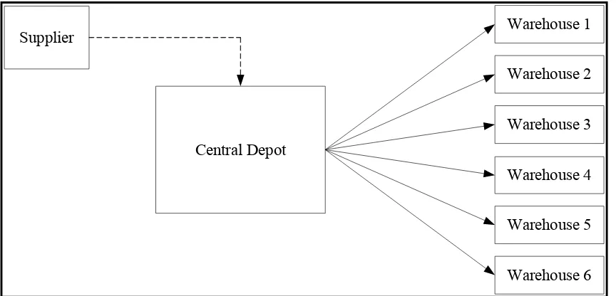
The case involve a company that markets tinned food for hotels, restaurants and catering segment which supply chain network consists of a central depot, three suppliers, and six warehouses. The concern in this final year project is to determine the impact of forecasting modeling on total cost performance, as a consequence of the type of data used in inventory management, of the central depot where stocks received, distributed, packaged, and sent to warehouses and the transportation cost for every replenishment trucks from suppliers. The problem layout is illustrated as in Figure 1.1.
In a simple term, the problem address by this project is to investigate the impact of forecasting modeling on the total cost associated with the inventory and transportation situation depicted in Figure 1.
Figure 1.1: The Problem Layout
Supplier
Central Depot
Warehouse 1
6 1.3Research Objectives
This project is dealing with an industrial situation as described in the problem statement with the ultimate objective to investigate the impact of the forecasting modeling selection transportation and inventory total cost, therefore the objectives of this project are
1. To fully understand the concept of demand forecasting practiced in the industry.
2. To fully understand the inventory policy that commonly used in industry.
3. To develop a mathematical model that can represent the transportation and inventory
carrying cost of the case described in the problem statement using MS Excel.
4. To conduct comprehensive computational works to determine the impact of
forecasting modeling on the inventory carrying cost and transportation cost.
5. To report the findings.
1.4Research Scope