PORTFOLIO MANAGEMENT:
MEAN-VARIANCE ANALYSIS I N THE US ASSET MARKET
Narela Spaseski
Depar tment of Economics, Inter national Univer sity of Sar ajevo, Hr asni cka Cest a 15, I lidza, 71200 Sar ajevo BiH, nar el [email protected]
ABSTRACT
n pr act ice an invest or would like t o have t he highest r et urn possible. However , asset s wit h high r et ur n usually cor r elat e wit h high r isk. The expect ed r et ur n and ri sk measur ed by t he var iance ar e t he t wo main char act er ist ics’ of a por t folio. Mean-var iance model as a good opt imizer can exploit t he corr elat ion, t he expect ed r et ur n, and t he r isk and user constr aint s t o obt ain an opt imi zed por t fol io. Alt hough it is t he simplest model of i nvest ment s, is suffi cient l y r ich t o be dir ect ly useful in applied pr oblems and decision t heor y.
In t he paper t wo met hods ar e present ed t hat exempl ify t he flexibilit y of it s applicat ion: maximi zing the r et ur n and minimizing t he ri sk. Based on t he numer i cal soluti on it can easily be under st ood that , for an i nvest or , specifying a t arget r et ur n may be mor e int uit i ve t han st r uggling with r isk aver sion coefficient. The pr oblems are formulat ed by using t he Wolfr am Mat hemat ical Progr ammi ng Syst em.
Key words: por t folio optimization, mean-var iance model and decision t heory.
1. Introduction
In practice an investor would like to have the highest return possible. However, assets with high return usually correlate with high risk. The expected return and risk measured by the variance are the two main characteristics’ of a portfolio. The behaviour of portfolio can be quite different from the behaviour of individual components of the portfolio. The risk of a constructed portfolio could be half the sum of the risk of individual assets in the portfolio. This is due to complex correlation patterns between individual assets. Therefore, we need a portfolio optimization.
Mean-variance model as a good optimizer can exploit the correlation, the expected return, and the risk and user constraints to obtain an optimized portfolio. Although it is the simplest model of investments, is sufficiently rich to be directly useful in applied problems and decision theory.
Since Markowitz published his seminal works on mean-variance portfolio selection in 1952 and 1968, his classical model has been serving as a basic of modern finance theory. The mathematical formulation of the Markowitz’s portfolio selection problem is the trade-off between risk and return which combines probability theory and optimization theory to model the behaviour of the economic agent. This is the first quantitative treatment of the theory and we cannot call it Modern Portfolio Theory (MPT) as some people, and use it as a main workforce on which analytical portfolio management is based. We should be very careful because this classical model is valid if the return is multi-variates normally distributed and the investor is averse to risk (prefers lower risk), or if for any given return which is multi-variates distributed the investor has quadratic objective function.
As Britten-Jones (1999) notes: “Mean-Variance analysis is important for both practitioners and researchers in finance. For practitioners, theory suggests that mean-variance efficient portfolios can play an important role in portfolio management application. For researchers in finance mean-variance analysis is central to many asset pricing theories as well as to empirical tests of those theories; however practitioners have reported difficulties in implementing mean-variance analysis.”
The difficulties in implementing this analysis in practice mainly arise as a result of the following four assumptions:
Single-period model. Meaning, investors can only make decisions at the beginning and must wait for the results without adjusting the portfolio weights until the end of the horizon. Preferences depend only on the mean and variance of payoffs
- At a given mean, lower variance is preferred
- At a given variance, a higher mean is preferred.
Price-taking with no taxes or transaction costs (known as the assumption of “perfect capital markets”)
Investors have enough historical data and that the situation of asset market in future can be correctly reflected by asset data in the past. But what if new assets are listed in the market, there is no past information for these securities.
2. Markowitz Mean-Variance Portfolio Theory
In Markowitz Mean-Variance Portfolio Theory the rate of return of assets are random variables. The goal is than to choose the portfolio weighting factors optimally. Meaning, the investor’s portfolio achieves an acceptable expected rate of return with minimal volatility. Here as a surrogate for the volatility is taken the variance of the rate of return.
Let us now consider constructing a portfolio consisting of n assets. We have an initial budget x0 that we wish to assign. The amount that we assign to asset i is x0i=wix0 for i=1,2,...n, where wi is weighting factor for asset i. What is also important to note, we allow the weights to take negative values. If a negative values accurse, the asset is being shorted in the portfolio. Therefore, to preserve the budget constraint we require that the weights sum to be 1, ∑ = 1. Thus, the sum of the investment is,
= =
The returns are also dependent on each other in a certain way and the dependence will be described by the covariance between them. The covariance between the i-th and the j-th return is denoted by,
σij = cov(Xi,Xj)=E(Xi-μi)(Xj-μj)
Note that in this notation, σij stands for the variance of the return of i-th asset,
σij = E(Xi-μi) 2
Meaning, given a universe of assets with random return Ri, i = 1, . . . , n , expected return μi, and covariance
matrix ∑= [σij], we should select portfolio weights wi adding up to one. Given a vector of weights representing the portfolio, its expected return and variance are given as follows:
− ∑ μ w = μ w, σ − wσ w − w ∑w Eq.1
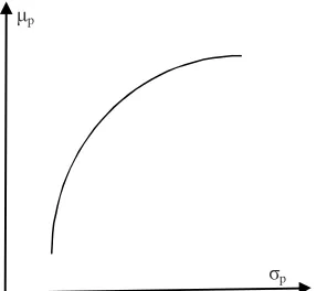
We continue the analysis by describing the set of all optimal portfolios known as the mean variance efficient portfolios. The standard deviation of return, σp might be considered as a risk measure, as it provides us with
a measure of dispersion. Actually, variance and standard deviation are interchangeable notions in this case.
Then, we may trade off expected return (μp) against risk (σp). Of course the trade off may be unclear, but it
can be visualized by tracing the frontier of mean- variance efficient portfolios, depicted in Fig. 1.
A portfolio is efficient if it is not possible to obtain a higher expected return without increasing risk or, seeing things the other way around, if it is not possible to decrease risk without decreasing expected return.
Figure 1. Mean- variance efficient portfolio frontier
σp
Now we are in position to state the optimization problem. The optimization problem behind the first
Similarly, the optimization problem behind the second formulation is,
2. max − ∑w
s.t. ∑ w = 1
wi≥ 0
3. Application
3.1. Data
The data used is obtained on the basis of Independent Investment Research, Morningstar (available online: http://www.morningstar.com/). We consider a sample of 8 assets with their monthly history of return for the period January 2012 - June 2014. The portfolio is composed of highly risky assets and less risky assets. Less risky assets are the following:
1. American Funds US Government Sec A AMUSX.
2. American Funds New Economy A ANEFX.
The remaining 6 assets listed below, are with higher risk.
3. USAA Mutual Fund Trust Precious Metals & Minerals Fund USAGX.
4. American Funds Bond Fund of Amer A BFABX.
5. T Rowe Price Equity Fund PRFDX.
Using Wolfram Mathematical Proagramming System we generate the following results:
As we can notice in Table 1, the USAGX asset is with variance 99.4055 and mean -1.451.Based on this information most of the investors will decide not to consider the asset 3 in their portfolio. But before drawing any final decision we should take in consideration the possible correlation between asset with the lowest risk (asset 1) and the asset with highest risk ( asset 3) .If the returns are negatively correlated (sigma <0) including asset 1 may, in fact, be beneficial in reducing risk. In our case the correlation is -0.681667. Meaning, the asset 1 will be included in the portfolio.
III.2.2.Mean-Variance model
The main goal behind the concept of mean-variance model is to combine various assets into portfolios and then to mange those portfolios so as to achieve the desired investment objectives. To be more specific, there are two main possibilities to make a sound decision: ether to minimize the risk or maximize the return.
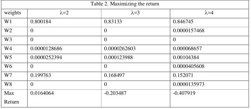
Quadratic programming model for portfolio optimization by risk factor 1 (maximize the return)
max − ∑w
s.t. ∑ w = 1
wi≥ 0
From a mathematical perspective, this is a Quadratic programming model. Coefficient l can be interpreted as a risk aversion coefficient. By changing the value of l, we can trace the efficient set. Unfortunately, it is a bit difficult to get a feeling for the parameter l. Anyway, common sense and experience suggest risk aversion coefficients in the range between 2 and 4. Therefore, we calculate the weights for three scenarios where is 2,3and 4see Table 2).
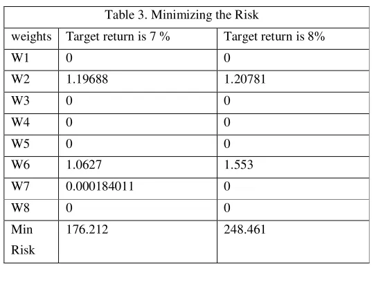
Quadratic programming model for portfolio optimization: constraint approach (minimize the risk) min wT∑w
s.t. wTμ = μi ∑ w = 1
Targeting the return to 7% and 8% we calculate the asset weights and risk (see Table 3). Accordingly, the investor can make an intelligent decision in which assets to invest as well as their weights.
Note:
- If we specify the return to 7% then the minimum risk is 176.212 and we should invest in asset 2, 6 and 7.
- If we specify the return to 10% then the minimum risk will be 248.461, and we should invest in asset 2 and 6.
4. Conclusion
Due to complex correlation patterns between individual assets, portfolio optimization is a key idea in investing. Mean-variance model as a good optimizer can exploit the correlation, the expected return, and the risk and user constraints to obtain an optimized portfolio. Therefore, application of Mean-Variance model is quite common and one of standard tools of decision making in both theory and practice. But we should be very careful because this classical model is valid if the return is multi-variates normally distributed and the investor is averse to risk (prefers lower risk), or if for any given return which is multi-variates distributed the investor has quadratic objective function.
In the paper two methods are presented that exemplify the flexibility of its application: maximizing the return and minimizing the risk. Based on the numerical solution provided in section 3, it can easily be understood that, for an investor, specifying a target return may be more intuitive than struggling with risk aversion coefficient.
Table 3. Minimizing the Risk
weights Target return is 7 % Target return is 8%
W1 0 0
W2 1.19688 1.20781
W3 0 0
W4 0 0
W5 0 0
W6 1.0627 1.553
W7 0.000184011 0
W8 0 0
Min
Risk
References
1. Ballestero, E. (2005). Mean-Semivariance Efficient Frontier: A Downside Risk Model for Portfolio Selection. Applied Mathematical Finance, 12(1),1-15.
2. Britten‐Jones, M. (1999). The Sampling Error in Estimates of Mean‐Variance Efficient Portfolio Weights. The Journal of Finance, 54(2), 655-671.
3. Deng, X.T., Li,Z.F., Wong,S.Y.(2005). A minimax portfolio selection strategy with equilibrium.
European Journal of Operation Research, 166,278-292.
4. Estrada, J. (2008). Mean-Semivariance Optimization: A Heuristic Approach. Journal of Applied Finance-Spring/Summer 2008: 57-72.
5. Estrada, J.(2006). Downside Risk in Practice. Journal of Applied Corporate Finance, 18(1), 117-125.
6. Grootveld, H. And Hallerbach, W.(1999). Variance vs downside risk: Is there really that much difference?. European Journal of Operational Research,114(2),304-319.
7. Hallow, W.V. (1991). Asset Allocation in a Downside-Risk Framework. Financial Analyst Journal, 47(5), 28-40.
8. Markowitz, H. (1952). Portfolio selection*. The journal of finance, 7(1), 77-91.
9. Markowitz, H. M. (1968). Portfolio selection: efficient diversification of investments (Vol. 16). Yale university press.