A model of a myelinated nerve axon thres

(1)

J. Math. Biology (1985) 23:119-135 Journal of

Mathematical

61ology

9 Springer-Verlag 1985

A model o f a myelinated nerve axon: threshold behaviour

and propagation

P. Grindrod* and B. D. Sleeman

Department of Mathematical Sciences, University of Dundee, Dundee DD1 4HN, U.K.

Abstract. A model o f a myelinated nerve axon is developed on the basis of F i t z H u g h - N a g u m o dynamics under the assumption that the nodes of Ranvier are of small but finite width. It is shown that a periodic excited state may not exist if the width of the nodes is too small and the leakage across the myelin sheath is too great. The propagation of a super threshold pulse is prevented

in the absence of nodes. Global stability of the resting equilibrium state is investigated as well as the propagation of "wave front", type solutions.

Key words: Myelinated nerve axons - - Nodes o f R a n v i e r - - F i t z H u g h - N a g u m o dynamics - - Threshold b e h a v i o u r - - Global stability - - Wave fronts

O. Introduction

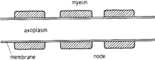
A myelinated nerve axon consists of a long cylindrical m e m b r a n e which is surrounded by a sheath of lipoprotein, called myelin, formed from a condensation of Schwann cell membranes. This fatty layered tissue insulates the axon from the external ionic fluid. At approximately millimetre intervals there are small gaps called nodes of Ranvier. These nodes expose the extracellular fluid to the excitable axon m e m b r a n e . At the nodes the axon m e m b r a n e is selectively per- meable to the charged ions within the a x o p l a s m and outer ionic fluid. Hence ionic currents m a y pass through the m e m b r a n e in the same way as for the somewhat simpler unmyelinated axon (see Fig. 1). Between the nodes the myelin sheath prevents ionic transport, except possibly for some leakage from the

Fig. 1. A myelinated nerve axon

myelin

axopbsm

~\ V/////////A V/////////~ V//////////~

\

membrane node

(2)

120 P. Grindrod and B. D. Sleeman

axoplasm, through the membrane, to small pockets of plasma held within the folds of lipoprotein. Stimulation at one node generates longitudinal ionic currents which excite neighbouring nodes. Because of the insulating nature of the myeli- hated segments impulses have the character of jumping from node to node. This form of conduction is referred to as saltatory conduction.

In that which follows we allow the nodes to have a finite longitudinal length and derive a model for the behaviour of the transmembrane potential along the axon.

The approach adopted in this paper differs from that of FitzHugh [4] and Bell and Cosner [2] who assume the nodes to be point sources of excitation. Here we are able to allow the node width to be as small as we please and use it as a parameter to control the degree of excitation possible at each node. In order to derive our model we consider equivalent electric circuits for the myelinated and unmyelinated segments separately and apply r - c cable theory.

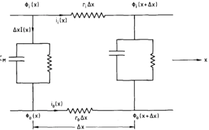
Figure 2 shows the equivalent circuit for a myelinated segment. Here ~ ( x ) and ~o(X) denote the longitudinal axoplasmic and external fluid potentials respectively; r~ and ro respectively denote the longitudinal resistivities of the axoplasm and external fluid and cm denotes the capacitance per unit length of the myelinated membrane.

I(x)

denotes the effective membrane current density while

i~(x)

and

io(x)

denote the longitudinal axoplasmic and external currents respectively. R denotes the resistivity of the myelinated membrane.

On applying Ohm's law and Kirchhoff's laws we obtain the following equation governing the transmembrane potential, viz. v = ~ - ~o where

1

Gray,

=

(ro+ r~) vxx

-

v/ R.

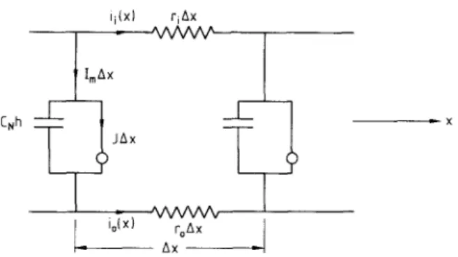
(0.1)

Figure 3 shows the equivalent electric circuit for a node segment. Here

J(x)

denotes the ionic current density present in the membrane at a distance x along the axon. It is this current which provides the excitation. We remark that energy is used up in driving such a current.

In this circuit CN denotes the capacitance per unit length of the membrane

(CN > CM).

(~i (X} r i AX

i~'• ' w v v w x ,

I

4~i(x+Z~x}

m •

io(x) ' w w v '

4'o (x) ro&x 4~o(x*Ax)

1

.4

(3)

Model o f a rnyelinated nerve axon ₁₂₁

Ci~h

ii(•

riA•

ImAX

"~JAx

F~

j

~

A

X

~

x

Fig. 3. An u n m y e l i n a t e d (node) segment o f nerve axon: the equivalent electric circuit

Again by applying Ohm's law and Kirchhoff's laws we obtain

1

CNV,

= Vxx -- J. (0.2)

to+ ri

In the model (0.2) we must specify the form of the ionic membrane current density J. Usually J is modelled by H o d g k i n - H u x l e y dynamics but this requires the introduction of three auxiliary variables which represent the rise and fall of the membrane permeability to sodium and potassium ions. Alternatively we may use the simpler F i t z H u g h - N a g u m o dynamics which have been successfully employed in the study of unmyelinated nerve axons. Thus we set

J= - f ( v ) + z ,

(0.3)

Z t = O - V - - ~ / Z ,

where o-, y are positive constants and

f(v)

is a non-linear function of v whose qualitative behaviour is shown in Fig. 4. For example we could take

f(v)=

v(1-v.)(v-a),

0 < a < 8 9 The dependent variable z represents the level of potassium permeability o f the membrane and serves as a recovery variable. Thus enabling the action potential to return to equilibrium after excitation.

In Eqs. (0.3) the constants or and 7 are usually small and the recovery equation for z is " s l o w " in comparison with the potential Eq. (0.2). Henceforth we shall not include the recovery process in the present model, but will instead restrict

Fig. 4. The qualitative form o f f

f(v)

(4)

122 P. G r i n d r o d a n d B. D. S l e e m a n

our analysis to the "excitory-phase" for the action potentials at the nodes. That is, we will use (0.2) together with

J = -f(v).

(0.4)

The same assumption is made in [2].

For the unmyelinated axon, the speed and shape of the leading front of propagating pulses may be approximated by a monotone travelling front obtained from the F i t z H u g h - N a g u m o equations without recovery (see [4]), so we may expect a similar approximation for myelinated axons to be attainable from the present model, (see Sect. 4). The "excitory-phase" should be strong enough to shift the transmembrane potential from rest up to some excited steady state, from where the recovery process would eventually return it to rest.

To complete the model we match equations (0.1), (0.2) across the myelin-node junctions by applying the following continuity conditions at a typical junction x =

X 0 9

(a) v(xo, t)l+_=-lim{v(Xo+e, t)-V(Xo-e,

t ) } = 0 ,

~ . - - . " 0

(0.5)

(b)

Vx(Xo, t)l+=-lim{vx(xo+e, t ) - v x ( x o - e ,

t ) } = 0 .

- e . . ~ O

Condition (0.5a) demands that the transmembrane potential v be continuous across junctions while (0.5b) follows from the local continuity of the longitudinal currents

ii(x)

and

io(x)

at x = Xo.

Once the positions and widths of the nodes have been specified we may use (0.1), (0.2), (0.4) and (0.5) to model an infinitely long myelinated axon. The simplest case to consider, and the one adopted in this paper is that in which the nodes have uniform width and are located at periodic intervals along the axon. Since the recovery process has been neglected a wave of excitation along the axon corresponds to a shift in the potential v away from the resting state (v = 0 in this case) to some positive excited state. We note that if recovery is incorporated in the model then this would return the potential to the resting equilibrium after some time.

We also expect to observe a threshold phenomenon. That is, if

v(x,

0) is small, then in either the "sup n o r m " or the L2-norm, the solution evolves to the zero resting equilibrium.

In Sect. 1 we investigate threshold behaviour and show that a periodic excited steady state may not exist if the width of the nodes is too small and the leakage across the myelin sheath is too great. In Sect. 2 we show how propagation of a superthreshold solution may be prevented in the absence of nodes. In Sect. 3 we derive an explicit condition on the system parameters which ensures that the resting equilibrium is globally stable. In all these cases we are in effect indicating how the nerve axon may degenerate. Finally, in Sect. 4 we discuss the propagation of "wave-front" type solutions. Such solutions travel with a constant speed along the axon, while the wave front profile oscillates with time.

(5)

Model of a myelinated nerve axon 123

Comparison theorem. Let g: ~ -~ [0, 1] be a continuous function satisfying g(O) =

g(1) = 0. Suppose u( x, t) and v( x, t) are continuously differentiable functions from R • R + to [0, 1] satisfying the differential inequalities

CNut - u~x - g(u) >i CNv, - Vx~ - g(v), for t>~O, x~(O, 0) mod(1),

CMut - u~ + u / R >! Csavt - Vxx + v / R

for t >>-O, x c (0, 1) mod(1), where 0 ~ (0, 1), CN, CM and R are positive constants. Then u(x, O) >1 v(x, O) for all x ~ R implies

u ( x , t ) > ~ v ( x , t ) f o r a l l x 6 R , t>~O.

The p r o o f of the above theorem follows in the same way as used by Aronson and Weinberger in [1], except that the continuity o f ut, vt and ux, vx must be used to show that v(x, t) - u ( x , t) cannot have a local m i n i m u m value o f zero at x = 0 or 0 mod(1).

1. Superthreshold steady-state solutions

Consider an infinitely long uniform myelinated axon and assume that the indepen- dent variable x has been scaled so that the nodes have width 0<< 1 located a distance 1 - 0 apart. F r o m the discussion o f the previous section the model takes the form of the initial value problem

CNu, = uxx + f ( u ) ,

CMu, = Ux~ - u / R ,

U(X, t)[ + = U~(X, t)]_ + = O,

x ~ ( O , O) mod(1), t~>O.

x ~ (0, 1) mod(1), t~>O, (1.1) x = O, 0 mod(1), t~>O.

where the initial data u(x, O) satisfies

0<~ u(x, 0)~< 1.

Here R > 0 is assumed to be large a n d f i s of the form described in the introduction. The c o m p a r i s o n theorem applied to (1.1) shows that [0, 1] is an invariant set for solutions u. That is 0~< u(x, 0)~< 1 for all x c ~ implies O<-u(x, t)<~l for all x c • , t~>0. I f u(x,O) is constant for all x then u(x, t) must converge to some 1-periodic steady state solution v(x) say where v(x) ~ [0, 1] for all x ~ R. Clearly v ~ 0 is one such solution and we wish to determine whether there are others. In particular we seek a super threshold steady state solution v(x) defined to satisfy condition A as follows.

Condition A

v ( x + l ) = v ( x ) , f o r a l l x ~ R and a<~v(x)<-I for all x ~ [0, 0]. That is, v(x) is 1-periodic and is stimulated by ionic m e m b r a n e currents at the nodes.

Since v(x) is a steady state solution o f (1.1) we have

Vx:,+f(v)=O, xE(O, O) mod(1). (1.2a)

v x x - v / R = O , x e ( O , 1) rood(l). (1.2b)

(6)

Let us consider the phase portraits for (1.2a) and (1.2b). These can be described in terms of the first order system of ordinary differenital equations

q~ = PN, (1.3a)

P% = -f(qN),

q ~ = P~' (1.3b)

P ~ = q~/R,

where '---

d~ dx

and the subscripts M, N refer to the myelinated and node segments of tile axon. Clearly a solution

v(x)

of (1.2) satisfying condition A is equivalent to two orbit segments, one from (1.3a) and one from (1.3b), joined together to form a closed loop. If the maximum of such a solution occurs on an orbit segment from (1.3b) then Vr, ax <~ 0. However the orbits of both (1.3a) and (1.3b) are strictly monotone decreasing for q < 0 , p ~< 0. Thus such an orbit segment from (1.3b) could never form part of a closed loop and so the maximum of a solution

v(x)

must occur somewhere on an orbit segment from (1.3a).

That is for

(qN, PN)

satisfying

PN

= 0, a < qN < 1. This argument also implies that the minimum must also occur on the positive q-axis since the orbits in both phase planes can never reach the negative q-axis from the lower half plane.

Lemma 1.1.

Any solution v(x) of

(1.2)

which is 1-periodic lies in the interior of

the triangular set

T = {(q, p)]0<~ q ~< 1, IP] ~<

q/v/R}, in the (q, p)-plane.

Proof:

We have seen that if

v(x)

exists then its maxima and minima must both lie in T. Suppose

(v(x), v'(x))

leaves r via an orbit segment from (1.3a) (i.e. for some x c ( 0 , 0) rood(l)). Then it must exit through the lower edge of T. However an orbit segment from (1.3b) cannot return

(v(x), v'(x))

to the upper half plane in this case and so v(x) will not be periodic. A similar argument eliminates the possibility of

(v(x), v'(x))

leaving T for

xe(O,

1)mod(1). This completes the p r o o f o f the lemma.

Lemma 1.2.

A solution v( x) to

(1.2)

satisfying condition A must also satisfy

v(O) = v(O)

mod(1),

and

v'(O) = -v'(O)

mod(1).

Proof.

A solution

(qN(S), pN(S))

of (1.3a) for s e (0, 0) satisfies

f qN a)

l ( p ~ ( s ) - p ~ ( 0 ) )

f(y) dy.

(1.4a)

= --~ qN(o)

Similarly a solution

(qM(s), pM(S))

of (1.3b) for s e (0, 1) satisfies

89

--pM(S)) 2) = f

qM(1)

(7)

Model o f a myelinated nerve axon 125

On setting s = 0 in (1.4) and using the continuity conditions at 0 and 0 mod(1) we obtain

~(p~( O) -p~,(O)) = l ( p ~ ( O) - P~,(O))

__ f qM(O)

f qN(O)

f ( y ) dy y / R dy - - - - j qM(O ) = J qN(O)

which implies that

q,~(o) (f(Y) + y / R ) dy = 0. (1.5)

M(o)

However qM(O), qM(O) c (a, 1) by condition A and so the integrand in (1.5) is strictly positive for y ~ (a, 1). Consequently we must have qM (0) = qM(0). Finally from the symmetry of the (q, p)-phase plane it follows that

PM( O) = PN( O) = --PM(O) = --PN(O)

as required.

Let us now return to the phase plane for (1.3a) and consider a solution

(qN(s), pN(s)) for s e (0, 0) satisfying

p,,(o)

=

-pN( o),

qN(O) = qN(O) = q say, where ~ e (a, 1).

On fixing ~ we may define the "time m a p " T for trajectories starting at (qN(0),pN(0)) = (~, p) (see Fig. 5a) as

T(p, #) = inf{s e R + IPN(S) = 0}.

This map is always of the form shown in Fig. 5b and we refer to [6] as a general reference for this kind o f analysis.

Here T(p, [1) is defined for p c (0, if) where fi is the pw-coordinate of the intersection of the stable manifold for (1, 0) and the line qN = q- Indeed

~2 = 2 f ( y ) dy,

and is a m o n o t o n e decreasing function o f ~ e (a, 1).

PN I

_I

F

~ \\ \\\

I \\\ \\~

a ~ 1 ~ qN

TIPN,q)

l

1

0 ~

b

Fig. 5. a (qN, pN)-phase plane, b The time map

(8)

Now for ~ e (a, 1) let s(p, ~) denote the "time" taken to reach the qM-axis,

and so

In other words

p*(~) = q~(O)

= ~

4~

tanh((1 - 0)/2v/R). (1.8)

Thus for fixed 0 we require ~ ~ (a, 1) such that T(~, p*) = 0/2.

By the symmetry of the phase-plane we have a solution v(x) of (1.2) satisfying the conditions

(i) v(0) = v(O) = ~ mod(1) (ii) v'(0) = - v ' ( 0 ) = p * mod(1)

(iii) v ( x ) = q ~ ( x ) of the form (1.7) for xe(O, 1)mod(1).

Conversely we see that if T(~, p*) # 0/2, with p* given by (1.8) for all ~ c (a, 1), then there cannot exist a solution v(x) of (1.2) satisfying condition A.

Theorem 1.3. For each fixed R > 0 there exists 0o> 0 such that if 0 < 0 < Oo then there are no solutions v(x) of (1.2) satisfying condition A.

Proof. Let M = maxu~(a.l)f(u), then since v(x)~ [a, 1] for x ~ (0, 0)mod(1) we have 0 i> v " - M . Thus for any ~ ~ (a, 1) and 16 > 0 the solution of (1.3a) which starts at (~,/~) satisfies

p(x)>~-Mx +16

and so p(x)>i 0 for x <~/~/M. Thus we have shown that the time map T satisfies

T(~, ~) > ~ / M for all 16 ~ (0,/~) and ~ e (a, 1). Since we require T(16, ~) = 0/2 we must have 16<~ MO/2. However along the corresponding trajectory we see from (1.7) that 16 must also satisfy

i6

= p*(~) = ~ tanh((1 - 0)/2x/--R).

V K

a

MO/2 >~ --~ tanh((1 - 0)/2x/-R). (1.9) via (1.3b), from the starting point

( qM( O ), p~( O ) ) = ( (1, - P ). (1.6) Then for every ~ c (a, 1) there exists p*(t~)>0 such that

1 - 0

= s ( p * ( ~ ) ,

~).

2

In fact the solution of (1.3b) subject to the condition (1.6) is given by q c o s h ( ( 2 ( s - 0 ) - (1 - 0))/2x/-R)

(9)

M o d e l o f a m y e l i n a t e d n e r v e a x o n 127

0.45

0.40

0,35

0.30

0.25

0,20

0.15

0,10

0,05

0.00

Fig. 6 0 2 4 8 i9

N o w as 0 ~ 0 the r i g h t - h a n d side o f (1.9) tends to a/v/-Rtanh(1/2~/R) thus violating the inequality. C o n s e q u e n t l y there exists 0o > 0 such that for 0 < 0o (1.9) ceases to h o l d a n d so no c o r r e s p o n d i n g solution v(x) o f (1.3a) exists. This completes the proof.

O n e c a n obtain an estimate o f 0o by sketching the zero c o n t o u r o f

MO a

F ( O , R ) - 2 x/--R tanh((1 - 0)/2x/~-)"

F o r a n y R > 0 a n d fixed F(O, R ) = 0 has a u n i q u e solution 0". Notice also that (1.9) implies 0 " ~ < 0o. T h u s if 0 < 0 " ~ < 0o then the c o n c l u s i o n o f t h e o r e m (1.3) holds. In Fig. 6 a g r a p h o f R versus 0* along the zero curve o f F(O, R) is given in which

f ( u ) : u(1 - u)(u - a), a n d a = 0.10, 0 . 1 1 , . . . , 0.20.

2. The N o n - e x i s t e n c e o f a propagating superthreshold action potential

In this section we c o n s i d e r a n o n - u n i f o r m m y e l i n a t e d axon. Specifically we consider the h a l f line p r o b l e m

C M U t = U x x - u / g , x ~ ( X b X i + l ) , /-even

(2.1)

Cuut = uxx +f(u), x e (Xi, X/+a), /-odd

where f ( u ) = u ( l - u)(u - a), Xo = 0 a n d limi_,oo Xi = co. The b o u n d a r y / i n i t i a l conditions are

u(0, t) = 1

(2.2)

(10)

To complete the model we impose the continuity condition

u(X,, t ) l + - = u,,(x~, t)l~ = o.

In this notation X~ (/-odd) denotes the position of the ( i + 1)/2th myelin-node junction and X~ (/-even) denotes the position of the i/2th node-myelin junction. To begin with we study the possible steady state solutions for (2.1), (2.2). Thus in the notation of the previous section we consider the systems

q ~ =PM

x ~ (Xi, Xi+l), /-even (2.3)

p'~ = qM/ R q'N = pN

X a (X~, Xi+l), /-odd (2.4)

P'N = - f ( q N )

By superimposing the phase-portraits for (2.3) and (2.4) on a single diagram we obtain the portraits shown in Fig. 7.

Suppose q~(0) = 1, q~(0) = ,/, then the solution to (2.3) for x ~ (Xo, X1) satisfying these conditions is

q ~ ( x ) = cosh(x/x/R)+ ~/x/R sinh(x/x/R),

p ~ ( x ) = R -1/2 sinh(x/x/-R)+ ~ / c o s h ( x / v ~ ) .

On eliminating ~ we see that the locus of ( q M ( x l ) , p ~ ( x l ) ) lies on the line 1

qM(XI) = ~ tanh( X1/ x/-R )pM( X1) -~ c o s h ( X l / q ~ ) (2.5) We are interested in the particular value of ( q ~ ( X t ) , p ~ ( X I ) ) which lies on the line

1

PM -- - ~ q ~ . (2.6)

Since (2.6) is a separatrix for the system (2.3) this can only happen when q~(0) = 1, pM(0) = - 1 / x / R = ~7.

Explicitly qM(X1) = exp(-X1/x/-R), p m ( X l ) = -1/x/-R exp(-XJx/-R).

f

P

I I p 1

__~ M = ~ q M

(11)

We have the following fundamental lemma. Lemma 2.1. Suppose, for X~/v/-R sufficiently large, that

f (q)

_{> 1 ,} _{q E (0, exp(-Xa/~/-R));}

q

then there exists a steady state solution to (2.3), (2.4) such that q(O) = 1, q(oo) = 0 and q'(x) <~ 0 for all x ~ R §

Proof. Define the set

So= {(q,p) iq =-- 1, -b<~p << - -1/vr-R for some b > 1/x/-R}. For 7 ~ So let y . x denote the solution o f

q'=p, x ~ R +,

p,=[q/v~,, x ~ ( X i , Xi+l), /-even (2.7)

t - f ( q ) , x~(X,,X,§

i-odd,

such that (q(0), p(0)) = 3'-

Observe that 3' is not a flow since

(3'. x) . y ~ 3'- ( x + y ) in general.

Nevertheless " . " is continuous on S o x R +. Now choose b so that ( 1 , - b ) . X1 lies on the stable manifold S -~, say, of (0, 0) for the phase portrait defined by (2.4). This is guaranteed by hypothesis, and we denote the q-component of (1, - b ) 9 X1 by q*. Furthermore, for all 3'~ So, the q-component of 3'. X1 lies to the left o f e x p ( - X ~ / v ~ ) .

For any interval I c R define

3". ~r= {3". x l x c S}.

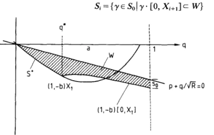
Next, let W be the closed set in the (q, p ) - p l a n e defined by W = {(q, p)/O <~ q ~ 1, p+qV'-R<~O, (q,p) lies above or on S + for O~q<~q * and lies above or on ( 1 , - b ) . [ O , X1] for q*~<q~<l} see Fig. 8. From Fig. 8 we see that So = W n {q = 1}. Now define

s, = {3'c Sol3'. [o, x , + , ] c w }

q* I

I

~ i a / 11

, w /

i

(1,-b) X ~ , - 7 ~ " ~ ~o_ -

(1,-b)[O,X~]

_--q

p + q/vrff=O

(12)

as depicted in Fig. 9.

We n o w m a k e the following observations.

(a) E a c h Si is n o n - e m p t y and closed. This follows since if i is o d d then there exists 3' ~ Si_l such that 3'. X~ is on S + and so 3'. X~§ is on S + c W. Similarly if i is even then there exists 3' ~ Si-1 for which 3'. Xi is on the line { p + q/x~--R= 0} n W e W. The h y p o t h e s i s o f the l e m m a is i m p o r t a n t here since it says that points in W subject to the flow g e n e r a t e d by (2.4) can only exit f r o m W along the line p + q/x/--R = 0. Since at least one point is on S § at x = X ~ ( - o d d ) and stays in W there exists a 3'o~So so that Yo" Xi+~ is on p + q/x/--R = 0. In other w o r d s 3'0" [0, X~+2] c W implies S~+1 (/-odd) is n o n - e m p t y .

(b) E a c h S~ is closed since W is closed a n d " 9 " is continuous. S~ D S~+1 for all i>~ 0, as is clear f r o m the definition o f S~.

S oo

F r o m (a) a n d (b) we m a y define = ('7~=o S~. Since S is the intersection of an infinite n u m b e r o f n o n - e m p t y closed sets satisfying (b) we have S ~ th.

N o w let 3' ~ S. T h e n 3'. x ~ (0, 0) as x--> oo. This follows since otherwise it leaves W at s o m e finite E but then 3' ~ S~ for i sufficiently large. We have thus s h o w n the existence o f a solution ( q ( x ) , p(x)) c o r r e s p o n d i n g to the initial value (q(0), p ( 0 ) ) = 3' and satisfying q(oo) = 0. This c o m p l e t e s the p r o o f of the l e m m a . Using L e m m a 2.1 t o g e t h e r with the c o m p a r i s o n t h e o r e m of Sect. 0 we have the result.

Theorem 2.2. Let

(i) q(x) be a steady state solution to (2.1) satisfying the hypothesis of Lemma

2.1.

(ii) u(x, t) be the solution to the problem (2.1), (2.2) for which the initial data h(x) satisfies

h ( x ) ~ q ( x ) .

Then u(x, t)<~q(x) for all (x, t ) ~ R + X R +. In other words u(x, t) remains sub- threshold (u(x, t) < a) at every node segment (Xi, X H ) , i-odd.

J

,/

9

~

p + ql4-R= 0

S2X31 SO SI S2

~ s 2 x ~ ~ -- _

i

SoX

1

i

I ,, I

m i i

(13)

3. Global stability of the resting equilibrium

In Sect. 1 it was s h o w n that if R is small or the u n i f o r m i n t e r n o d e distance 0 is small then the only p e r i o d - o n e steady state solution is u =- 0. H e r e we shall analyse the stability o f this solution using the c o m p a r i s o n t h e o r e m o f Sect. 0 a n d a spectral t h e o r y a r g u m e n t .

We c o n s i d e r the C a u c h y p r o b l e m (1.1) a n d a s s u m e for simplicity cm =- cN = 1. To begin with define

s = s u p { f ( u ) / u } a n d g = l / R ,

u ~ 0

where f ( u ) is o f the f o r m s h o w n in Fig. 4. I n d e e d i f f ( u ) = u(1 - u)(u - a) then s = (1 - a)2/4. We next define the function q(x) by

- s f o r x c [ 0 , 0 ] r o o d ( l )

q(x) = g for x ~ (0, 1) r o o d ( l ) , and s u p p o s e that w(x, t) satisfies the C a u c h y p r o b l e m

w, = w x x - q ( x ) w , (x, t ) c R x R + (3.1) where w(x, O) >>- u(x, 0) ~> 0 for all x ~ •.

F r o m the c o m p a r i s o n t h e o r e m of Sect. 0 it is clear that

w(x,t)>~u(x,t) f o r a l l ( x , t ) E ~ x ~ + where u(x, t) is the solution to the C a u c h y p r o b l e m (1.1).

Theorem 3.1. Suppose the quantities s, g and 0 satisfy the inequality n =- g ( 1 - o ) - Os, > 0

then the resting equilibrium u-~O of Eqs. (1.1) is asymptotically stable in

L2(R), i.e.

Ilu(.,

t)ll <~ c ent.

Proof. T h e idea o f the p r o o f is to show that the equilibrium solution w = 0 to (3.1) is a s y m p t o t i c a l l y stable which t o g e t h e r with the c o m p a r i s o n t h e o r e m will i m p l y the a s y m p t o t i c stability o f (1.1).

Define

D = {v c L2(R): v'(x) exists is a b s o l u t e l y c o n t i n u o u s on R and

- v " + q(x)v c L2(R)}. For v ~ D define the linear o p e r a t o r

d 2

Lv = (--~xz + q(x) ) v.

It is easy to verify that (i) L is self-adjoint

(ii) the s p e c t r u m or(L) o f L is real and p u r e l y c o n t i n u o u s (iii) A ~ tr(L) implies A ~> (1 - O ) g - Os.

For details o f this and related matters see [3].

N o w w(x, t) satisfies w, + Lw = 0 and by the a b o v e r e m a r k s L is an infinitesimal g e n e r a t o r o f an analytic s e m i - g r o u p {e-Lt}, t ~> 0. It follows f r o m [5] that there exists a c o n s t a n t C such that

(14)

132

This estimate together with the hypothesis that

Os - g(1 - 0) < 0 implies the result.

P. Grindrod and B. D. Sleeman

4. Propagation of wave-front like solutions

In this section we shall study the existence o f propagating front like solutions to (1.1). Since R >> 0 we choose to approximate our model by the simplification

u , = u x x + a ( x ) f ( u ) , ( x , t ) ~ R x R + (4.1) where f ( u ) = u(1 - u ) ( u - a), 0 < a < 89 and a ( x ) is a non-negative periodic function of period one such that

a ( x ) = l f o r x e ( 0 , 0 ) m o d ( 1 )

= 0 otherwise. (4.2)

Equation (4.1) always admits a superthreshold steady state solution u --- 1, so we do not encounter any of the degenerate cases discussed in Sects. 1-3.

N o w we will assume that a ( x ) in (4.1) has the form a ( x ) = ~ + e f t ( x ) , where t~ > 0 and f t ( x ) is a uniformly continuous 1 periodic function of x and satisfies

o f t ( x ) d x = 0 .

Consider the equation

Yz~ - Cyz + 6 f ( y ) = 0 (4.3) It is well k n o w n that for a e (0, 89 (4.3) has a front solution r satisfying

lim Oh(z) = 0

z - ~ - - c o

lim ~b(z) = 1

z - - > or3

ck'(z)>>-O for all z, if and only if c = x / - ~ ( 1 - 2 a ) / x / 2 .

In (4.1) we set u(x, t ) = ( a ( z ) + p ( z , t), where z = x + c t , it follows that

P, = Pz~ - cpz + 5 ( f ( p + r - f ( c k ) ) + e f t ( z - c t ) f ( p + r )

together with the conditions limlzl_,oo p(z, t ) = 0 for all t. N o w set p = eQ, then

Qt = Qz~ - cQz + 6f'(q~ )Q + [3 (z - c t ) f ( ga) + O ( e ) .

To order e, Q satisfies the linear perturbed equation

(15)

Model of a myelinated nerve axon 133 It can be shown that the spectrum of A contains an isolated simple eigenvalue at the origin, with eigenfunction r and that the remaining eigenvalues and essential spectrum are bounded to the right of the imaginary axis (see [5], p. 131, for example).

Lemma 4.1. I f fl0 •(X) dx = O, then (4.4) has a solution Qo(z, t) such that

(a) Qo(z, t) ~ BCo for all t ~ R.

(b) Qo(z, t ) = Q ( z , t+ 1 ) f o r a l l t ~ R .

Proof. The proof of the lemma rests on a general result concerning periodic solutions for periodically forced parabolic equations, which will be published elsewhere [7]. The point is that (4.4) has a solution Qo satisfying (a) and (b) above if and only if

f l/c

0 = P[fl(z - c t ) f ( r dt

dO

where P is the projection of BCo onto the linear subspace spanned by r fl/c

Since P is linear this is certainly true when Jo f l ( z - c t ) dt = O, and the lemma follows.

Immediately we have

Theorem 4.2 I f a ( x ) = ~ + eft ( x ), where 6 > 0 and ~ ~ fl ( x ) dx = O, then for all e ~ ~,

(4.1) has a solution of the form

u(x, t) = if(z, t) = r t)+ O(e2), (4.5)

where r is the front solution of (4.3), and Qo is given by Lemma 4.1.

In particular when e is small then the function (4.5) approaches a travelling front solution with an oscillatory profile in time.

Remarks. 1. Although the above result applies only when e > 0 is assumed small numerical evidence suggests that such solutions exist when a ( x ) is an arbitrary

1-periodic non-negative function (and in particular the step function introduced in (4.2)).

We conjecture that if a ( x ) is any non-negative one-periodic function with average 6 =~1 o a ( x ) d x , then (4.1) admits a travelling front type solution with speed c = v/-6(1-2a)/,r and a time-oscillating profile of period 1/c.

Figures 10 and 11 depict such solutions for a = 0 . 1 and a ( x ) = 3 2 for x ~ [0, 0.25)mod(1) and zero otherwise. In these figures we have changed to the variables (z, t) so that the solutions appear to be standing oscillatory fronts.

(16)

d

" 0 " 0

o

" 0

{3

- - o o o o

o o

o

=.

o'-

c~

i _ o--

c~

i

a -

<5

' o

~J

o

o~

(17)

Acknowledgments. The authors thank Dr B. P. Rynne for many helpful discussions and Miss J.

Patterson for carrying out the numerical experiments reported in Sect. 4.

References

1. Aronson, D. G., Weinberger, H. F.: Nonlinear diffusion in population genetics, combustion and nerve pulse propagation. In: Partial differential equations and related topics. Lect. Notes Math., Vol. 446. Berlin, Heidelberg, New York: Springer 1975

2. Bell, J., Cosner, C.: Threshold conditions for a diffusion model of a myelinated axon. J. Math. Biol. 18, 39-52 (1983)

3. Eastham, M. S. P.: The spectral theory of periodic differential equations. Scottish Academic Press, 1973

4. FitzHugh, R.: Mathematical models of excitation and propagation in nerve fibres. In: Schwan, H. P. (ed.) Biological Engineering. New York: McGraw-Hill 1963

5. Henry, D.: Geometric theory of semilinear parabolic equations. Lect. Notes Math., Vol. 840. Berlin, Heidelberg, New York: Springer 1981

6. Smoller, J. A., Wasserman, A.: Global bifurcation of steady-state solutions. J. Differ. Equations 39, 269-290 (1981)

7. Grindrod, P., Rynne, B. P.: Time-periodic solutions of semilinear parabolic equations. University of Dundee Applied Analysis Report AA846 (1984)