Volterra Series identification Based on State Transition Algorithm with Orthogonal Transformation

(1)

DOI:_{10.12928/TELKOMNIKA.v14i1.2663} ₁₇₁

Volterra Series identification Based on State Transition

Algorithm with Orthogonal Transformation

Cong Wang*1, Hong-Li Zhang1, Wen-hui Fan2 1

College of Electrical Engineering, Xinjiang University Urumqi Xinjiang， 830047, China 2

Department of Automation, Tsinghua University, Beijing 100084, China *Corresponding author, email: 641087385@qq.com

Abstract

A Volterra kernel identification method based on state transition algorithm with orthogonal transformation (called OTSTA) was proposed to solve the hard problem in identifying Volterra kernels of nonlinear systems. Firstly, the population with chaotic sequences was initialized by using chaotic strategy. Then the orthogonal transformation was used to finish the mutation operator of the selected individual. OTSTA was used on the identification of Volterra series, and compared with particle swarm optimization (called PSO) and state transition algorithm (STA). The simulation results showed that OTSTA has better identification precision and convergence than PSO and STA under non-noise interference. And when there is noise, the identification precision, convergence and anti-interference of OTSTA are also superior to PSO and STA.

Keywords: State Translation Algorithm; Orthogonal Transformation; Nonlinear System; Volterra Series; System Identification

1. Introduction

More and more high coupling nonlinear system appaered for the development of high technology, how to describe these models has been become a research hotspot. With the development of the nonlinear theory, Volterra series has been widely applied in the modeling and faults diagnosis of nonlinear system [1]. Volterra functional series considers the dynamic characters of the system, and its kernel has a distinct physical meaning. So the series can approximate arbitrary precision continuous function on the set, and describes the categories of nonlinear phenomenon [2].

The key of building nonlinear system by Volterra series model is to identify the structure and parameter of the model [3]. So, there is an urgent demand for effective identification methods.

The traditional identification methods on Volterra series generally adopt the least squares algorithm [4], but the least squares’ identification efficiency is relatively low and easy to fall into local minimum. In recent years, intelligent optimization methods has been introduced into the kernel identification on the Volterra series problems, like genetic algorithm [5], adaptive ant colony algorithm [6], quantum particle swarm optimization [7-8], cross-correlation method [9], etc. Those algorithms can overcome the drawbacks of the traditional identification methods, such as the requirement on the continuous differentiable objective function, and the sensitivity the measurement noise. However, they still have their own limitations on solving the problem of optimization [10]. Consequently, none of these algorithms can accurately solve the problem of Volterra series identification.

(2)

the conflict between convergence speed and global search capability efficiently and so facilitate diversity within the population, improving the global search ability of the algorithm.

2. Volterra Series

The single input and output nonlinear system can be expressed by Volterra series[11] as the follows:









1

1 0 0 1

y , ,

k

n k k m

k i i m

h i i u n i            _  _  

  

L L



(1)

Here,

u n

 

and

y n

 

are the input and output of the system respectively,

h i

_k



₁

,

L

,

i

_k



is the kth-order time domain kernel of the system [7].

The first three orders with the Volterra series is generally used to describe the dynamics characteristics of nonlinear system. The kth-order time domain is unique and symmetric. With its symmetry, the Volterra series is shown as Equation (2):

 

  



    

 





 

  

1 2

3 1 2

1 1 1

1 2 0 0 1 1 1 3 0 , , , , , , ] i

N N N

i i j i

N N N

i j i k j

y n h i u n i A i j h i j u n i u n j

B i j k h i j k u n i u n j u n k e n

                 _{ }         _



 

  

(2)

Here,

 

_, 1

2,

if i j A i j

if i j

    _  ， ,









 



1

, , 6, (

3,

if i j k

B i j k if i j j k i k if else      _      I I ， ,



1, 2,3



p

N

p



is the Volterra kernel memory length, and

e n

 

is the truncation error.

 



  

  



 





2

2 3 2 3

, , 1 , , 2 1 , ,

( 1), , 3 ( ) 1 , , ( 1) T X n x n x n N x n x n x n

x n N x n x n x n x n N

  _    _        _ _ L L L (3)



   

















1 1 2 2 2 3

3 3 3 1

h (0), , ( 1), 0, 0 , 0,1 , , 1. 1), h 0, 0, 0 ,

0, 0,1 , , 0, 0, 1 , , 1, 1, 1 T M

H h N h h h N N

h h N h N N N

      _        L L L L （ (4)

Where, N represents the kernel memory length. The system input vector is X(n), and kernel vector is H . Equation (2) describes the relationship between input and output of the nonlinear system, which can be expressed as the vector form, as follows:

 

T

   

y n H X n e n

(5)

It can be seen from Equation (5) that the output of a nonlinear system can be expressed as a linear combination of each element of the input vector X(n). The Volterra series model based nonlinear system identification is used to solve the kernel vector H when the input and output sequence of the system are given. The essence of the identification is a parameter optimization process.

(3)

3. Orthogonal Transformation State Transition Algorithm 3.1. State Transition Algorithm

The state transition algorithm was proposed by YANG in 2011 [12-14]. A solution to the specific optimization problem can be described as a state, and the optimization algorithm can be treated as state transition. Then the process to solve the optimization problem can be regarded as a state transition process.

The state transition algorithm is easy to understand, due to the less numbers of the parameters and the simple algorithm structure. The state transition is defined as the following form:

1

( ) k k k k k

k k

x A x B u

y f x



 



 _

 ₍₆₎

Here,

x

_k



R

nstands for a state and corresponds to a solution of the optimization

problem.

A

_k

，

B

_k



R

nn are state transition matrixes which can be regarded as the operators of optimization algorithm.

u

_k



R

nis the function of the state

x

_k and its history state. f is the objective function.

3.2. The Transition Operators

There are three operators called rotation transformation (RT), translation transformation (TT), expansion transformation (ET) in STA. Rotation transformation is used to improve the global search ability, translation transformation can improve local search ability, and expansion transformation can balance the relations between the two. Besides, reference [15] proposed axesion transformation to simplify the search ability of one dimensional.

The details of the four operators are shown as follows [15]: (1) Rotation transformation:

1

2

1

k k r k

k

x x R x

n x



   (7)

(2) Translation transformation:

1 1

1 2

k k

k k t

k k

x x x x R

x x

 





 

 (8)

(3) Expansion Transformation:

1

k k e k

x

_

 

x



R x

(9)

(4) Axesion Transformation:

1 a

k k k

x _  x 



R x (10)

Here,

x

_k



R

n,    ，，， are all positive constants, called rotation factor, translation factor, expansion factor, and axesion factor respectively.

R

_r



R

n n is a random matrix with its

elements belonging to the range of [-1, 1] and

2

k

x

is 2-norm of a vector.

R

_t



R

is a random

variable with its elements belonging to the range of [0,1].

R

_e



R

n n is a random diagonal matrix

n n

(4)

The procedure of the original state transition algorithm can be outlined as follows.

1: Initialize feasible solution x(0) randomly, set    ，，， and k ← 0 2: repeat

3: k=k+1

4: while



≤ error do

5: State ←Rotation transformation (x k( 1) _{, times of search enforcement,}α₎

6: if min f State( ) f x k( ( 1)) then 7: Updating x k( 1)

8: State ←Translation transformation (x k( 1), times of search enforcement, β) 9: if min f State( ) f x k( ( 1)) then

10: Updating x k( 1)

11: end if 12: end if

13:  ← c

f 

14: end while

15: State ←Expansion Transformation (x k( 1), times of search enforcement, ) 16: if minf State( ) f x k( ( 1)) then

18: State ←Translation transformation (x k( 1), times of search enforcement, β) 19: if minf State( ) f x k( ( 1)) then

21: end if 22: end if

23: State ←Axesion Transformation (x k( 1)_{, times of search enforcement,}



₎

24: if minf State( ) f x k( ( 1)) then 25: Updating x k( 1)

26: State ←Translation transformation (x k( 1)_{, times of search enforcement,}β₎

27: if minf State( ) f x k( ( 1)) then 28: Updating x k( 1)

29: end if 30: end if 31: x k( ) ←x k( 1)

32: until the specified termination criterion is met

3.3. Orthogonal Transformation Strategy

In order to further enhance the algorithm's searching ability, the state transition algorithm based on the orthogonal transform (OTSTA) is proposed. In OTSTA chaotic strategy is used to initialize the population for its nonrepeatability and ergodicity. The orthogonal transformation operation is applied on the poor individuals during the process, which can effectively avoid premature convergence and improve the global search ability.

3.3.1. Initializing

In non-linear system, chaos is a common motion phenomenon with such excellent characteristics as ergodicity, randomness and “regularity”.Chaotic motion can experience all the states in the state space without repetition according to certain “rule” within certain motion range [16]. During initialization, firstly chaotic strategy is used to randomly generate M dimensional vector

X

₁



（

x

₁₁

,

x

₁₂

,



,

x

₁_M

)

. Then, the model iterative chaotic sequence containing N vectors is obtained by the Logistic map [17], shown in Equation (11).

1

=

(1

),

0,1,...,

1

k k k

(5)

Here,





（

0, 4],

x



[0,1]

.In this paper, we use the same parameter setting



=4

as [17, 18]. The fitness values of all the states are calculated by fitness function. Then better performance part is chosen as the initial solution.

Using chaotic sequence to initialize states improves the diversity of the states without lose of randomness.

3.3.2. Orthogonal Transformation Strategy

In order to maintain the diversity and breadth of search, this paper adopts the orthogonal transformation along with the original four operators. About 10% individuals D t( )

with the poor fitness value are chosen from the overall size P(t) after each completed state transformation. Then orthogonal matrix X is gotten through orthogonal transformation under the orthogonal basis. For anyxD t( ), if the orthogonal x’ has better fitness value, x would be replaced by x’. Otherwise, x would be preserved. The orthogonal operation is repeated until all chosen poor individual are replaced.

For any

 

,



x

_k, there is



x' , '



x



 



 

,



. x’ is called the orthogonal transformation of

x

_k. And

x

'

 



x

'

.Here



is the orthogonal basis of

x

_k.

4. Volterra Series Identification by OTSTA

The essence of Volterra series identification is that it could convert the parameter identification problem to optimization problem. STA is used to find function optimal solution and to get the minimum evaluation function value. The kernel vector H of Volterra series, which needs to be identified, is seen as the state Xk of OTSTA, and the state transition is

regarded as the process of identification algorithm.

For Volterra series identification problem, the square of the difference between the actual output and the parameter model output is set to be the evaluation function of Volterra series identification, shown in Equation (12):

 









2

1

L i

J h y k i y k i 





_   %  _ (12)

Here, L is the length of the window, and

y k

%

 

is the estimated output value. The algorithm

demonstrates the whole process of OTSTA:

OTSTA

Step 1 Initialization:

 Initialize initial state by chaotic sequence

 Set parameters

 Calculate the fitness value based on equation(8)

Step 2 Iteration

 Execute strategy: RT,ET,AT

 If get better fitness value, execute TT, else maintain

Step 3 Updating the status



1

(

_k

)

f x

_ <

f x

( )

_k ,

x

_k_₁ instead of

x

_k,else

x

_k

maintain

Step 4 Use Orthogonal transformation

 OT used on 10% individual with poor values

 maintain better state

best x



Step 5 Replace



best x



replaces the current state

step 6 End

 Meet the requirement, end

(6)

5. Performance Evaluation

We considered the following second order nonlinear model as the experimental subject [19]:

2 2

y( ) 0.5 ( ) 0.4 (n  u n  u n 1) 0.9 (u n2)+1.2 ( ) 0.2 (u n  u n 1) 0.8 (u n1) (u n2) ₍₁₃₎

According to the Volterra theory, the kernel vector of the nonlinear system was H= [0.5,-0.4, 0.9, 1.2, 0, 0, 0.2,-0.8, 0].

The white noise signal was chosen as the system input. The variance was set as 1 and the length was set as 20. In order to verify the search ability and search speed of the OTSTA, the input and output with or without noise were both considered when using the second order Volterra to build the nonlinear model. In order to test the performance of the proposed algorithm, STA, PSO and Reference [19], which were recognized as distinguished algorithms for Volterra series identification, were used for comparison with OTSTA.

The OTSTA was used to identify the kernel vector of Volterra series without noise whose parameters were set as follows on the basis of experimental method:

a) Times of search enforcement : 500, b) The number of epoch: 100,

c) Communication frequency : 50Hz, d)



: 1 to e-5,

e)   、、 : 1, f)

f

_c: 5.

In order to ensure fairness, the STA was set the same parameters as OTSTA. The parameters of PSO were set through many times test as follows:

a) The number of particle : 100, b) The number of iterations : 500, c) Contraction factor s : 0.72, d) Accelerating factor: c1=c2=1.49.

We used the average deviation to evaluate the stability of three algorithms.

10

i 1 av.dev = T*T





(14)

*

T

is the value that the actual value minus simulation value, T is the actual value.

5.1. Under No Noise Interference

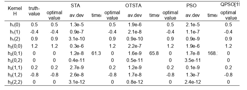
Programs were run independently for 20 trails for each algorithm in MATLAB R2010a The comparison results for OTSTA, STA, PSO and QPSO [19] were listed in Table 1. The convergence curve of OTSTA under no noise interference was shown as Figure 1. Figure 2 and Figure 3 showed the convergence curves of the Volterra kernel vector h1(0) and h2(0,0) of PSO，OTSTA and STA respectively. The truth-values were h1(0)=0.5，h2(0,0)=1.2.

Table 1. The results under the free-noise interference

Kernel H

truth- value

STA OTSTA PSO QPSO[19

optimal

value av.dev time/

optimal

value av.dev time/

optimal

value av.dev time/

optimal value

h1(0) 0.5 0.5 1.3e-5

61.3

0.5 1.9e-6

65.8

0.5 2.1e-5

168.2 0.5

h1(1) -0.4 -0.4 0.9e-7 -0.4 2.1e-8 -0.4 1.1e-7 -0.4

h1(2) 0.9 0.9 3.1e-10 0.9 0.9e-10 0.9 0.9e-9 0.9

h2(0,0) 1.2 1.2 0.3e-6 1.2 2.2e-7 1.2 1.9e-6 1.2

h2(0,1) 0 0 1.2e-8 0 1.6e-9 0 1.7e-8 0

h2(0,2) 0 0 0.4e-11 0 0.5e-11 0 3.5e-11 0

h2(1,1) 0.2 0.2 2.7e-9 0.2 1.2e-9 0.2 0.1e-9 0.2

h2(1,2) -0.8 -0.8 2.6e-8 -0.8 1.7e-8 -0.8 1.3e-7 -0.8

(7)

It can be seen from the Table 1 that OTSTA is superior to STA and PSO in Volterra series identification under no noise. It not only had fast convergence speed, but also had strong global search ability. Under no noise interference, OTSTA had no obvious advantage compared with QPSO in Reference [19].

Figure 1. The convergence curve under no noise interference

The preference of the algorithms was judged by the parameters identification error [20]. It can be seen from Figure 1, Figure 2 and Figure 3 that OTSTA can get the optimal solution when the iteration number up to 100, which means OTSTA had a better convergence and higher precision in identification on the Volterra series.

Figure2. The convergence curves of the Volterra kernel vector h1(0)under the no noise

interference

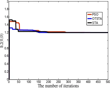
Figure 3. The convergence curves of the Volterra kernel vector h2(0,0)under the no

noise interference

5.2. Under Noise Interference

For the noisy case, the noise of superposition added on the input and the output was independent stationary white noise and its signal SNR was 20 dB.

The noise was added on the input and output respectively. We used the same methods. The results of the three algorithms and Reference [19] were shown in Table 2. The convergence curve of OTSTA under noise interference was shown in Figure 4. It can be seen from optimal value, av.dev and simulation time in table2 that OTSTA still had fast convergence speed and strong global search ability than STA and PSO under noise interference. And OTSTA was notable superior than Reference [19] in av.dev.

0 50 100 150 200 250 300 350 400 450 500 0

0.02 0.04 0.06 0.08 0.1 0.12 0.14 0.16 0.18

The number of iterations

T

h

e ou

tp

ut

e

rro

r

0 50 100 150 200 250 300 350 400 450 500 0.2

0.3 0.4 0.5 0.6 0.7 0.8

h1(

0

)

STA OTSTA PSO

0 50 100 150 200 250 300 350 400 450 500 0.6

0.8 1 1.2 1.4 1.6 1.8 2

h2(

0,

0

)

(8)

Table 2 The results of three algorithms under the noise interference

Kernel H

truth- value

STA OTSTA PSO QPSO[19]

optimal

value av.dev time/

optimal

value av.dev time/

optimal

value av.dev time/

optimal

value av.dev time/

h1(0) 0.5 0.49 2.1 e-3

76.3

0.49 1.8e-4

79.1

0.51 2.2e-3

188.5

0.49 9.7e-3

NaN

h1(1) -0.4 -0.41 0.3e-3 -0.40 0.1e-4 -0.4 1.2e-3 -0.40 3.7e-3

h1(2) 0.9 0.90 1.4e-2 0.90 2.2e-3 0.90 1.9e-3 0.90 7.0e-3

h2(0,0) 1.2 1.18 4.3e-2 1.21 1.1e-3 1.18 2.7e-2 1.18 2.0e-2

h2(0,1) 0 0 1.5e-3 0 3.6e-4 0 1.1e-3 0 1.6e-3

h2(0,2) 0 0 0.7e-3 0 0.4e-3 0 0.5e-3 0 0.4e-3

h2(1,1) 0.2 0.21 2.9e-3 0.2 4.3e-4 0.19 0.1e-2 0.19 0.6e-3

h2(1,2) -0.8 -0.8 1.8e-3 -0.8 1.7e-3 -0.83 2.3e-2 -0.78 1.7e-2

h2(2,2) 0 0 3.1e-4 0 1.5e-4 0 1.9e-3 0 1.4e-3

Figure 4. The convergence curve under noise interference

Figure 5 and 6 showed the changes in Volterra kernel vector h1(0) and h2(0,0) with number of iterations using the three algorithms, which described the convergence characteristics of the three algorithms in the optimization process. The OTSTA algorithm could converge and produce good optimization results after a small number of iterations, demonstrating convergence characteristics significantly better. PSO and STA had fluctuated obviously and slowly convergence speed by noise influenced.

Figure 5. The convergence curves of the Volterra kernel vector h1(0)under the noise

interference

Figure 6. The convergence curves of the Volterra kernel vector h2(0,0)under the noise

interference

0 50 100 150 200 250 300 350 400 450 500

0 0.02 0.04 0.06 0.08 0.1 0.12 0.14 0.16

T

h

e out

pu

t

er

ror

0 50 100 150 200 250 300 350 400 450 500

0 0.1 0.2 0.3 0.4 0.5 0.6 0.7 0.8 0.9 1

h1

(0)

PSO OTSTA STA

0 50 100 150 200 250 300 350 400 450 500

0 0.2 0.4 0.6 0.8 1 1.2 1.4 1.6 1.8 2

h2

(0

,0

)

(9)

From the analysis of the comparison of the above figures and tables, we know that OTSTA is a suitable tool to solve the volterra series identification under no noise as well as noise interference. It is not only has high precision, but also has Strong robustness.

6. Conclusion

Based on the the analysis on the principle and the kinematical characteristics of Volterra series, a new improved intelligent algorithm is proposed with orthogonal strategy. The chaotic strategy is used to initialize the population with chaotic sequences, and orthogonal transformation is used to transform mutation on some poor individuals, which can improve the global search ability. This improved state transition algorithm is applied to identify Volterra series, and the results are analyzed comparing with STA and PSO. Through the simulation experiment, OTSTA algorithm achieves higher identification precision than STA and PSO, and has higher identification speed than PSO under no noise as well as noise interference. State transition algorithm with orthogonal transformation is used on the identification on the Volterra series. This method can not only improve the global search capability effectively, avoid premature convergence, but also can maintain simple structure and has high search efficiency of state transition. This paper verifies that the OTSTA is feasible on nonlinear system Volterra kernel identification. The method provides a new effective method for nonlinear system identification.

Acknowledgements

The work was supported by the National Natural Science Foundation of China (Grant No. 51575469) and the Outstanding Doctor Graduate Student Innovation Project of Xinjiang University (No. XJUBSCX-2015014).

References

[1] Xia X, Zhou J, Xiao J, et al. A novel identification method of Volterra series in rotor-bearing system for fault diagnosis. Mechanical systems and signal processing. 2015; 66-67: 557-567.

[2] Kacar S, Cankaya I, Boz AF. Investigaton of computational load and parallel computing of Volterra series method for frequency analysis of nonlinear systems. Optoelectronics and advanced materials-rapid communications. 2014; 8(5-6): 555-566.

[3] Li NZ, Feng XY. Identification of Volterra series based on grey clustering multi-subpopulation adaptive PSO algorithm. Application Research of Computers. 2014; 31(6): 1697-1701.

[4] Peng ZK，Lang ZQ. The Nonlinear Output Frequency Response Function of One-Dimensional Chain Type Structure. ASME-Journal of Applied Mechnics. 2010; 77(1): 11007-11016.

[5] Tang H, Liao YH, Cao JY, et al. Fault Diagnosis Approach Based on Volterra Models. Mechanical Systems and Signal Processing. 2010; 24(4): 1099-1113.

[6] Li ZN, Tang GS, Xiao NX. Volterra series identification method based on adaptive ant colony optimization. Journal of Vibration And Shock. 2011; 30(10): 35-38.

[7] Li NZ, Feng XY. Volterra series identification method based on adaptive quantum-behaved particle swarm optimization combined with the chaotic strategy. Journal of Lanzhou University (Natural Sciences). 2014; 01: 128-135.

[8] Li ZN, Jiang J, Feng FZ. Hidden markov model recognition method based on Volterra kernel identified with particle swarm optimization. Chinese Journal of Scientific Instrument. 2011; 32(12): 2693-2698. [9] Orcioni S. Improving the approximation ability of Volterra series identified with a cross-correlation

method. Nonlinear Dynamics. 2014; 78(4): 2861-2869.

[10] Qiang ZY, Wu FP, Dong JR, et al. Optimization of power system scheduling based on shuffled complex evolution metropolis algorithm. TELKOMNIKA (Telecommunication Computing Electronics and Control). 2015; 13(2): 413-420.

[11] Wen XL, Chen Y. Research of the nonlinear system identification based on the volterra rls adaptive filter algorithm. TELKOMNIKA. 2013; 11(5): 2277-2283.

[12] Zhou XJ, Yang CH, Gui WH. Initial version of state transition algorithm. International Conference on Digital Manufacturing and Automation (ICDMA). 2011: 644-647.

[13] Zhou X J, Yang CH, Gui WH. Gui Wei-hua. State transition algorithm. Journal of Industrial and Management Optimization. 2012; 8(4): 1039-1056.

(10)

[15] Zhou XJ, Yang CH, Gui WH. Gui Wei-hua. A new transformation into state transition algorithm for finding the global minimum. International Conference on Intelligent Control and Information Processing (ICICIP). Harbin. 2011: 674-678.

[16] WU Ya-lin, ZHANG Shui-ping. A self-adaptive chaos particle swarm optimization algorithm. TELKOMNIKA (Telecommunication Computing Electronics and Control). 2015; 13(1): 331-340.

[17] Cao SH, Xu HM. Analysis of logistic map and chaotic sequence characteristics. Journal of Yanbian University (Natural Science). 2014; 40(2): 134-137.

[18] Binabaj FB, Farhangfar H, Azizian S, et al. Logistic regression analysis of some factors influencing incidence of retained placenta in a holstein dairy herd. Iranian Journal of Applied Animal Science. 2014; 4(2): 269-274.

[19] Li ZN, Liang J, Chan JG, Wu GH, Li XJ. Volterra series identification method based on quantum particle swarm optimization. Journal of vibration and shock. 2013; 32(3): 60-74.