Feedback Linearization Control for Path Tracking of Articulated Dump Truck

DOI: _{10.12928/TELKOMNIKA.v13i3.1810}  ₉₂₂

Feedback Linearization Control for Path Tracking of

Articulated Dump Truck

Xuan Zhao1, Jue Yang*1, Wenming Zhang1, Jun Zeng2 1

School of Mechanical Engineering, University of Science & Technology Beijing, Beijing, China

2

School of Computer and Communication Engineering, University of Science & Technology Beijing, Beijing, China, Telp：+86-010-62332467

*Corresponding author, e-mail: zhaoxuan120@126.com

Abstract

The articulated dump truck is a widespread transport vehicle for narrow rough terrain environment. To achieve the autonomous driving in the underground tunnel, this article proposes a path following strategy -for articulated vehicle based on feedback linearization algorithm. First of all, the kinematic model of articulated vehicle, which reflects the relationship between the structure parameters and state variables, has been established. Referring to the model, the nonlinear errors equation between real path and reference path, which are as the feedback from the path tracking process, has been solved and linearized. After estimating the system controllability, the path following controller with feedback linearization algorithm has been designed through calculating the parameters with the pole assignment according to the error equation. Finally, the Hardware-In-the-Loop simulation on NI cRIO and PXI controller has been -conducted for verifying the control quality and real-time path tracking performance. The result shows that the path tracking controller with feedback linearization can track the reference path accurately.

Keywords: articulated vehicle, path tracking, feedback linearization, hardware-In-the-loop

Copyright © 2015 Universitas Ahmad Dahlan. All rights reserved.

1. Introduction

The articulated dump truck is a transport vehicle which is widely used in mining, water conservancy and construction. It especially adapts to the narrow space, rough terrain and severe weather, for example, the tunnel in the underground mining. The autonomous driving system, an advanced automatic technology, can improve the vehicle productivity, operator safety and exhaust cleanliness [1]. The purpose of this article is to find a path following strategy for autonomous driving system on articulated vehicle.

Before developing the path following strategy, the articulated vehicle model, path following algorithm and controller test method need to be clear. The articulated vehicle modeling and path following control application have been investigated in many studies. In [2-4] kinematic model of articulated vehicle and error model between real and reference path are presented, and the path tracking simulation with model predictive control is applied, while in [5] the feedback controller based on Lyapunov approach is designed and the stability of the closed-loop system is proved in theory. The simulations in these literatures are non-real-time and the real-time performence has not been verified. Moreover, in [6] a trajectory tracking strateagy fora new structure automated guided vehicle is presented, while in [7] a feedback linearization control for almost global output-feedback tracking is provided for the underactuated autonomous quadrotor. Both the literatures have designed the controller of feedback linearization. However, the models of the plants are distinct from the articulated vehicle. This article need to design a path following algorithm controller with a kinematic model of articulated vehicle and test in a real-time environment.

in which the velocity of the front frame is considered as a measurable variable. Furthermore, the articulated vehicle model, as a highly nonlinear model, is hard to control. However, the feedback linearization can simplify the controller design. Meanwhile, controller real-time performence is important, while traditional offline simulation method cannot test. Hardware-In-the-Loop simulation is thus conducted toverify the real-time performance [8].

In this article, a 35 tons underground articulated mining truck with electical transmission designed by University of Science & Technology Beijing is selected as the research prototype. In Section 2, a kinematic model of the articulated vehicle has been builtthrough the geometrical relationship. In addition, the definition of the errors between real path and reference path has beendiscribed and modelled. In Section 3,according to the feedback linearization method, the state equation and output equation of the nonlinear articulated vehicle have been transformed to a linear controllable and observable system. Then the controller has been configured by linear control method to control the model for the precise path tracking. In Section 4, the Hardware-In-the-Loop simulation devices have been shownand the simulation procedure with different platforms have been introduced. In Section 5, the simulation has been launched to verify the quality of the controller. The results have been shown with the graphs. And the interpretation of the results has been discuss. In Section 6, the conclusion presents the findings of this article.

2. Articulated Vehicle Kinemics Modeling 2.1. Articulated Vehicle Mathematical Model

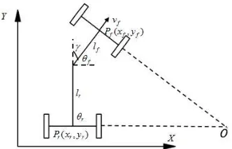
The articulated vehicle turning state is presented in Figure 1. In this figure, O is the instantaneous center of movement. Pf(xf,yf) and Pr(xr,yr), denote the corresponding center points of tractor and trailer. lfand lr are the length of the front and rear units. θfandθr denote the units orientation. γis the articulated angle which is defined as the difference between the front and rear orientation. Usually, considering simplifying calculation, Pf is the whole vehicle reference point, because the velocity vf orientation of this point is coincident with the whole vehicle orientation [9]. The velocity of articulated vehicle is defined as

f

vv (1)

Figure 1. Articulated vehicle scheme

The coordinates of Pf is:

cos

sin

f f f

f f f

x

v

y

v













(2)

The rate ofθf is composed of the angular velocity in constant radius turning and yaw velocity in fixed Pf pivot steering.

sin

cos

f r

f

f r

v

l

l

l

















The articulated vehicle state equation Pf=[xf,yf,θf,γ] is: 0

cos

0 sin

sin

cos cos

0 1

f f

f f

r f

f r f r

x y

l v

l l l l

















   

     

     

     

   _   _ 

     

  _ _ _ _

 

 



(4)

2.2. Path Description

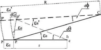
Figure 2 shows the errors between the real and reference path. The small circle of which the center is cis the real vehiclepath, while the big circle of which the center is C is the reference path. Ideally, the vehicle should passP1,P2,P3. The variables are defined as:

a) Lateral displacement error d:the lateral displacement errorbetween the vehicle reference point pand the corresponding point P (the nearest point on the reference path);

b) Orientation error :the orientation error between the velocity orientation of p and the tangential orientation of P;

c) Curvature error c: the curvature error between the curvature of p and P.

Figure 2. Articulated vehicle plan-view

2.3. Error Modeling

Figure 3 is a part of Figure 2. When the vehicle moves from p to p’, it revolves dθ around instantaneous center c at radius r. Radial lines cp and Cp’ intersect the reference path circle at P and P’ respectively. The angle between CP and CP’ is denoted d .

Figure 3. Geometric relationship of errors

a) Lateral displacement error d

Assuming both dθand d are small angles, the change of lateral displacement error is

d

Substituted with v=rdθ/dt, then the rate of lateral displacement error is:

d

v











(6)

b) Orientation error

According tothe geometric relationship,

d



_



d





d



(7)

(

R





_d

)

d





rd



(8)

From equation(7)(8), the steady-state steeringdifferential of orientation error is

1 d r d d R 







   _  _ 

  (9)

Generally, the width of the tunnel is about 5 m and width of the vehicle is 3.4 m. So d≤0.6 m, while the vehicle steering radiusr≤6.6 mthat means R≥6.6 m. Thus, assume thatR≫ d. Andconsidering the additional yaw angle velocity when





≠0, as well as substituting for v=rdθ/dt

and c=r -1

-R-1, the rate of orientation error is:

cos r c r f l v l l 









    _ _   

  (10)

c) Curvature error c

Known vehicle velocity v and reference path radius R, the real path radius is: cos sin r f f r l l v r v v l









    _{  }   

 _ (11)

Differentiatingreciprocal of Equation (11) with respect to time t gives,

 

1 2

2 2

( cos ) ( cos ) ( sin )

( cos ) ( cos )

f r r r f f r

c

r f r f

d r v l l l l l l l

dt v l l v l l

          _{  }        

 (12)

From Equation (6), (10), (12), the linearized state equation is:













1 1 1 0

0 0 0

0 0 cos 0

0 0 0

cos cos

d d

r r f

c c

r r f

r f v

v l l l

l v l l

l l            _{ }                   _    _{ }  _                            _  _{ } _  _{ }      (13)

Known-0.25π<γ<0.25πfrom vehicle structure, an assumption is made thatγis a small angle measured in radians and L=lf+lr. Redefine Equation (13) asthe articulated vehicle state equation for path tracking SMC design.

1

1

0 0 0

0 0

0 0 0

d d

r

c c

v

v l L

3. Feedback Linearization Control Algorithm Design 3.1. Feedback Linearization Method

Feedback linearization is a common method used in controlling nonlinear systems. The approach involves coming up with a transformation of the nonlinear system into an equivalent linear system through a change of variables and a suitable control input. The state feedback is implimented on the basis of vehicle kinematic model.The nonlinear kinematic model can be transformed into a closed-loop linear system via introducing appropriate state feedbacks. The well-established linear control theories are then applicable for the nonlinear systems with state feedback.

Moreover, the feedback linearized systems are observable as well as controllable. A linear control method is then proposed in order to control the vehicle kinematic model.

3.2. Controller Design

Before designing the controller, the system controllability must be estimated. If the rth derivative of system can express the relationship between output y(t) and input u(t), r is defined as the relative degree. The system is controllable when r≤n where n is system degree [11].

Analytically, from equation(14), c can be controlled by





and can be controlled by





and c as well as d can be controlled by . Thus, the articulated vehicle system is controllable when the articulated angle rate





is as the input. Assuming that the state variable vector

x=[ d, , c] T

is measurable, the path tracking controller can be designed with the state variable feedback [12].

Theoretically, the closed-loop system can be formatted as wish. The state feedback is denoted as u=-Kx, where Kis feedback gain and K=[k1,k2,k3]. The optimization objective is to find an appropriate K that can lead any arbitrary x to the desired value in time [13].

Supposed that the object controlled is a linear time-invariant time system expressed with state space equations as follow[14]

x AxBu (15)

The linear feedback is:

Kx

u   (16)

( )

x AB K x ₍₁₇₎

Where            0 0 0 0 0 0 0 v v

A , 1

1

0

r

B

l L

L

 









 











,























c d

x







 ,

u







,

K



[ ,

k k k

1 2

,

3

]

.

The system transition performance should be considered, such as response time, setting time and overshoot. The pole assignmentis the solution. In this article, differential transformation method is used for assigning the pole to the arbitrary location on plane S for system stability and transition performance. So the closed-loop pole can be set on the desired location in order to keep the system having 2nd order dynamic response that natural frequency

ωn and damping ratio ξis dominant. Meanwhile, the 3rd pole should be far away for these two poles on the left side half open complex plane S [15].

Considering the closed-loop stability of this system, the eigenvalue sof the eigenmatrix

A-BKis on the left side of plane S [16].

3 2 3 2 1 2 1 2

(

l k

r

k

)

(

l k

r

k

)

k

0

s

s

v

s

v

L

L

L













(18)

The truck sizes are lf=1.68m andL=5.12m and it drives with the constant velocityv=3 m/s. Solving the Equation (18), the State feedback gain can be obtain as:

1 2 3

[ , , ] [0.7, 3.9,15.6 ]

4. Hardware-In-the-Loop Simulation

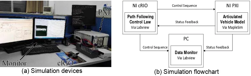
Hardware-In-the-Loop is a form of real-time simulation. Hardware-In-the-Loop differs from pure real-time simulation by the addition of a “real” component in the loop.This component may be an electronic control unit (ECU for automotive, FADEC for Aerospace) or a real engine. The purpose of a Hardware-In-the-Loop simulation is to provide all of the electrical stimuli needed to fully exercise the ECU. In effect, “fooling” the ECU into thinking that it is indeed connected to a real plant.In this article the component is NI cRIO as a path following controller. In this article,the Hardware-In-the-Loop devices are shown in Figure 4(a) and flowchart is in Figure 4(b). It shows that the plant, articulated vehicle modelled by MapleSim, is simulated in PXI and the cRIO controller, in which program is compiled by LabView, is real. To observe directly, all the data is uploaded to a PC to display with a graphical user interface programmed by LabView.

(a) Simulation devices

Path Following Control Law

Via Labview

Articulated Vehicle Model

Via MapleSim

Data Monitor Via Labview

Control Sequence

Status Feedback

Control Sequence Status Feedback

(b) Simulation flowchart

Figure 4. Hardware-In-the-Loopsimulation

5. Results and Discussion

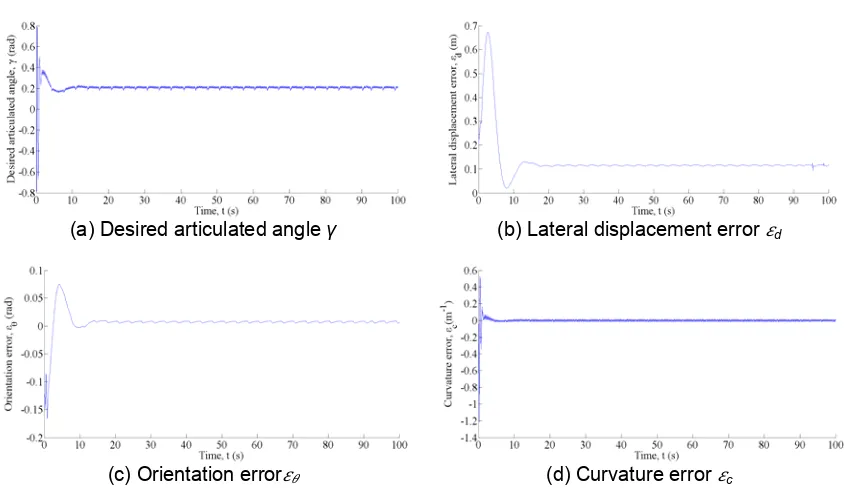
During the simulation, the truck follows a circle path with radius r=25 m in the constant speed v=3 m/s. The original point of the globle coordinate system is on the centre of the circle path. The starting point is (-3,-25), and the initial direction is -∞ of X axle.The simulation duration is 100 secends.

Figure 5. Contrast between reference and real path

(a) Desired articulated angle γ (b) Lateral displacement error d

(c) Orientation error (d) Curvature error c

Figure 6. Articulated angle and errors change

5. Conclusion

In this article, the research prototype is a 35-tonne electrical transmission underground mining articulated dump truck. And the hardware in the loop simulation is based on NI cRIO and PXI controller. The feedback linearization is used for designing the path tracking controller.

The conclusions of this article are:

a) For articulated vehicle model, a highly nonlinear model,the feedback linearization controllercantrack the reference path accurately. Both the dynamic and steady characteristicscan fulfill the demand.

b) The feedback linearization controller developed by the kinematics model can control the vehicle to follow the reference path without accurate dynamic model. The real path is smooth and little chattering.

Acknowledgements

This work was financially supported by the National High Technology Research and Development Program (863 Program) of China, under Awards 2011AA060404 Intelligent Underground Mining Truck.

References

[1] Dragt BJ, Camisani-Calzolari FR, Craig IK. An Overview of the Automation of Load-Haul-Dump Vehicles in an Underground Mining Environment. Proceedings of the 17th World Congress the International Federation of Automatic Control. Prague. 2005; 16: 1388-1400.

[2] Nayl T, Nikolakopoulos G, Gustfsson T. Switching Model Predictive Control for an Articulated Vehicle under Varying Slip Angle. 20th Mediterranean Conference on Control & Automation (MED). Barcelona. 2012: 890-895.

[3] Lee JH, Yoo WS. Predictive Control of a Vehicle Trajectory Using a Coupled Vector with Vehicle Velocity and Sideslip Angle. International Journal of Automotive Technology. 2009; 10(2): 211-217. [4] Ridley P, Corke P. Load Haul Dump Vehicle Kinematics and Control. Journal of Dynamic Systems,

Measurement, and Control. 2003; 125(1): 54-59.

[5] Petrov P, Chakyrski D. Path Following Control of an Articulated Mining Vehicle via Lyapunov Techniques. 17th NNTK International Conference. Sofia. 2009: 396-400.

[6] Ye X, Wu Z, Zhao F. Research on a 3 DOF Automated Guided Vehicle based on the Improved Feedback Linearization Method. 33rd Chinese Control Conference (CCC). Nanjing. 2014: 184-188. [7] Maithripala DHS, Berg JM. Robust Tracking Control for Underactuated Autonomous Vehicles Using

Feedback Linearization. Proceedings ofIEEE/ASME International Conference on Advanced Intelligent Mechatronics (AIM). Besancon. 2014: 446-451.

[8] Jackson R, Sarwar S. PXI Addresses New HIL Applications. Evaluation Engineering. 2005; 44(6): 24-28.

[9] Pei XZ, Liu ZY, Pei R. Application of Exact Feedback Linearization to Trajectory Tracking for Mobile Robot. Robot. 2001; 23(7): 661-680.

[10] Yuan L. Missile Attitude Control System Based on Trajectory Linearization. PhD Thesis. Harbin: Harbin Engineering University; 2013.

[11] Mahindrakar AD, Banavar RN. Controllability Properties of a Planar 3R Underactuated Manipulator. IEEE Conference on Control Applications. Glasgow. 2002: 489-494.

[12] Akhtar A, Nielsen C. Path Following for a Car-like Robot Using Transverse Feedback Linearization and Tangential Dynamic Extension. Proceedings of the IEEE Conference on Decision and Control. Orlando. 2011: 7974-7979.

[13] Song XJ. Design and Simulation of PMSM Feedback Linearization Control System. Telkomnika - Indonesian Journal of Electrical Engineering. 2013; 11(3): 1245-1250.

[14] Liu D, Zhou D, Liu Y. A Method of Multi-rate Single-side Networked control for Linear Time-Invariant System with State-feedback. 5th International Conference on Computer Science and Education (ICCSE). Hefei. 2010: 1270-1274.

[15] Hardiansyah, Junaidi. Multiobjective H2/H∞ Control Design with Regional Pole Constraints.

TELKOMNIKA Telecommunication Computing Electronics and Control. 2012; 10(1): 103-112.