CHARACTERISATION OF DATA SET FEATURES FOR STORAGE SPACE
OPTIMISATION USING FUNCTIONAL DEPENDENCY
PENYELIDIK:
DR. NURUL AKMAR EMRAN
DR. NORASWALIZA ABDULLAH
NUZAIMAH MUSTAFA
FAKULTI TEKNOLOGI MAKLUMAT DAN KOMUNIKASI
TABLE OF CONTENTS
PAGE
ABSTRACT ii
ACKNOWLEDGEMENT iii
LIST OF TABLES iv
LIST OF FIGURES v
LIST OF ABBREVIATIONS vi
CHAPTER 1 1
INTRODUCTION 1
1.1 Background 1
1.2 The Proxy-based Approach 2
1.3 Functional Dependency 4
1.4 Problem statement 6
1.5 Research Questions 7
1.6 Aims and Objective 7
1.7 Research Contribution 7
CHAPTER 2 8
LITERATURE REVIEW 8
2.1 Background 8
2.2 Application of Functional Dependency in different domain 8
2.2.1 Methods for FDs discovery 9
2.3 Data Incompleteness problem: Missing values 16
2.4 Conclusions 17
CHAPTER 3 19
MATERIALS AND METHODS 19
3.1 Background 19
3.2 Research Methodology 19
3.3 Data source of Microbial Genomics data sets 22
3.2.1 Description of the semantics of Taxon table attributes 24
3.2.2 Observation of missing values in Taxon table 25
3.4 TANE Algorithm for discovery of FDs 26
3.3.1 TANE Algorithm categories 27
3.5 The method in preparing analysis of space requirement 31
3.5.1 Proxy based approach for space optimisation 32
3.6 Conclusions 34
CHAPTER 4 35
RESULTS 35
4.1 Background 35
4.2 Proxy discovery from Taxon sub-tables 35
4.2.1 Summary output of table AE_F 46
4.2.2 Summary output of table AE_G 49
4.2.3 Summary output of table AE_H 52
4.2.5 Summary output of table AE_J 60
4.2.6 Summary output of table AE_K 63
4.2.7 Summary output of table AE_L 67
4.3 Summary of Space requirement results 71
4.3.1 Multi-valued table for Table AE_F 71
4.3.2 Multi-valued table for Table AE_G 72
4.3.3 Multi-valued table for Table AE_H 72
4.3.4 Multi-valued table for Table AE_I 73
4.3.5 Multi-valued table for Table AE_J 74
4.3.6 Multi-valued table for Table AE_K 75
4.3.7 Multi-valued table for Table AE_L 76
4.4 Conclusions 77
CHAPTER 5 78
RESULTS ANALYSIS AND DISCUSSIONS 78
5.1 Background 78
5.2 Analysis of FD accuracy for candidate proxy in Taxon sub-tables 78
5.3 Space Requirement Analysis 84
5.4 Conclusions 86
CHAPTER 6 87
CONCLUSIONS 87
REFERENCES 89
ABSTRACT
ACKNOWLEDGEMENT
Praise to Allah s.w.t for the strength, patience and endurance to complete this research. We would like to acknowledge Universiti Teknikal Malaysia Melaka for the financial assistance granted to pursue this research, the Faculty of Information and Commuication Technology and the Centre for Research and Innovation Management (CRIM). Without these bodies, the achievement of the objectives set for this research is not possible.
LIST OF TABLES
TABLE TITLE PAGE
Table 1: Types of dependencies ... 5
Table 2. List of attributes in Taxon ... 20
Table 3. Statistics of missing data in Taxon table ... 26
Table 4. A Proxy map in pure relational table (Emran, Abdullah, and Isa 2012) ... 33
Table 5. A Proxy map in a multi-valued table (Emran, Abdullah, and Isa 2012) ... 33
Table 6. FDs discoveries in AE_F table with G3 ranges of 0.10 to 1.00 ... 46
Table 7. Overall FD accuracy and proxy table size analysis for table AE_F ... 48
Table 8. FDs discoveries in AE_G table with G3 ranges of 0.10 to 1.00 ... 49
Table 9. Overall FD accuracy and proxy table size analysis for table AE_G ... 51
Table 10. FDs discoveries in AE_F table with G3 ranges of 0.10 to 1.00 ... 52
Table 11. Overall FD accuracy and proxy table size analysis for table AE_H ... 55
Table 12. FDs discoveries in AE_F table with G3 ranges of 0.10 to 1.00 ... 56
Table 13. Overall FD accuracy and proxy table size analysis for table AE_I ... 59
Table 14. FDs discoveries in AE_F table with G3 ranges of 0.10 to 1.00 ... 60
Table 15. Overall FD accuracy and proxy table size analysis for table AE_J ... 62
Table 16. FDs discoveries in AE_F table with G3 ranges of 0.10 to 1.00 ... 63
Table 17. Overall FD accuracy and proxy table size analysis for table AE_K ... 66
Table 18. FDs discoveries in AE_F table with G3 ranges of 0.10 to 1.00 ... 67
Table 19. Overall FD accuracy and proxy table size analysis for table AE_L... 70
Table 20. Multi-table scheme of table AE_F (total instances) ... 71
Table 21. Multi-table scheme of table AE_G (total instances) ... 72
Table 22. Multi-table scheme of table AE_H (total instances) ... 72
Table 23. Multi-table scheme of table AE_I (total instances) ... 73
Table 24. Multi-table scheme of table AE_J (total instances)... 74
Table 25. Multi-table scheme of table AE_K (total instances) ... 75
Table 26. Multi-table scheme of table AE_L (total instances) ... 76
Table 27. Overall summary of FD accuracy percentage for candidate proxies. ... 78
Table 28. Proxy candidates that do not shows any accuracy in FD prediction ... 79
LIST OF FIGURES
FIGURE TITLE PAGE
Figure 1: An example of substitution made by proxy attribute B for attribute D ... 3
Figure 2(a) A database instance violating ∑ = {cnt, arCode reg, cnt, reg prov}. (b) An optimum V-repair (Kolahi & Lakshmanan, 2009) ... 10
Figure 3. An example of an unclean database and possible repairs. (George, et al., 2010) ... 11
Figure 4. Example of various types of repairs. (George, et al., 2010) ... 12
Figure 5. Sample inconsistent databases (Molinaro and Greco 2010). ... 14
Figure 6. Sample consistent databases (Molinaro and Greco 2010). ... 14
Figure 7. Flow chart of overall methodology ... 22
Figure 8. TANE main algorithm (Adapted from Huhtala et al., 1999) ... 28
Figure 9. Generating levels algorithm (Adapted from Huhtala et al., 1999) ... 29
Figure 10. Computing dependencies algorithm (Adapted from Huhtala et al., 1999) ... 29
Figure 11. Pruning the lattice algorithm (Adapted from Huhtala et al., 1999) ... 30
Figure 12. Computing partitions algorithm (Adapted from Huhtala et al., 1999) ... 30
Figure 13. Approximate Dependencies algorithm (Adapted from Huhtala et al., 1999) ... 31
Figure 14. Output of TANE algorithms for table AE_F on 0.10 G3 range ... 36
Figure 15. Output of TANE algorithms for table AE_F on 0.20 G3 range ... 37
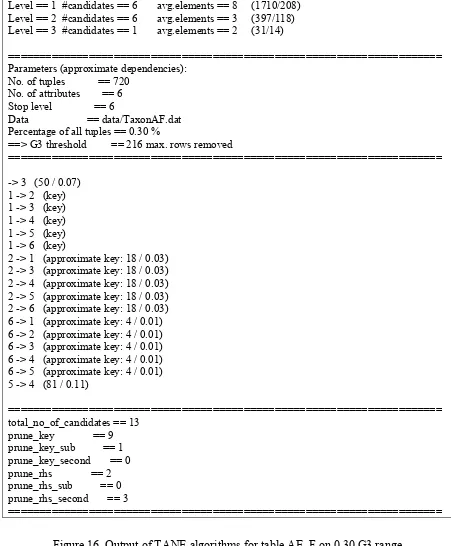
Figure 16. Output of TANE algorithms for table AE_F on 0.30 G3 range ... 38
Figure 17. Output of TANE algorithms for table AE_F on 0.40 G3 range ... 39
Figure 18. Output of TANE algorithms for table AE_F on 0.50 G3 range ... 40
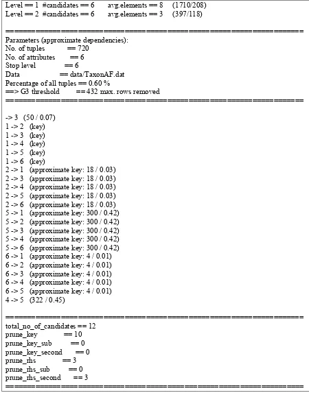
Figure 19. Output of TANE algorithms for table AE_F on 0.60 G3 range ... 41
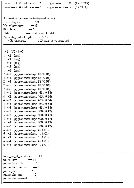
Figure 20. Output of TANE algorithms for table AE_F on 0.70 G3 range ... 42
Figure 21. Output of TANE algorithms for table AE_F on 0.80 G3 range ... 43
Figure 22. Output of TANE algorithms for table AE_F on 0.90 G3 range ... 44
Figure 23. Output of TANE algorithms for table AE_F on 1.00 G3 range ... 45
Figure 24. FD accuracy percentage and G3 errors table AE_F ... 80
Figure 25. FD accuracy percentage and G3 errors for table AE_G ... 81
Figure 26. Proxy H FD accuracy percentage and G3 errors table AE_H ... 81
Figure 27. FD accuracy percentage and G3 errors table AE_I... 82
Figure 28. FD accuracy percentage and G3 errors table AE_J ... 82
Figure 29. FD accuracy percentage and G3 errors table AE_K ... 83
Figure 30. FD accuracy percentage and G3 errors table AE_L ... 83
LIST OF ABBREVIATIONS
FDs - Functional Dependencies
CHAPTER 1
INTRODUCTION
1.1 Background
1.2 The Proxy-based Approach
Within the context of applications that require access to databases, data volumes often be large enough for storage space requirements to become an issue that must be dealt by data center providers. Expanding database storage is an option that data center providers could take in order to address the space issue, however this option leads to an increase in the amount of physical data storages (data servers) required.
One way to reduce storage space requirement is by optimising the available database space. In fact, the need to optimise space is not new, as tools and techniques for this purpose provided by enterprise data storage vendors (such as Oracle and DB2) have been available in the market for about a decade. At the relational table level, data compression tools, for example, apply a repeated values removal technique to gain free space (Lai, 2008). In addition, data deduplication techniques remove duplicate records in the table to gain storage space (Freeman, 2007). The idea behind these space optimisation solutions is to exploit the presence of overlaps (of values or records) within tables. Both of these techniques are performed at the level of whole tables. A key (though often unstated) assumption behind these optimisation techniques is that all columns can be exploited for space optimisation. Because of this assumption, knowledge of semantics of applications (i.e., how the columns are used) is ignored and as the consequence, data center providers need to bear unnecessary query processing overhead for frequent compression (and decompression) of heavily queried data.
In this research, we propose a space optimisation technique called the proxy- based approach. The proposed technique will be designed by exploiting the functional
dependencies discovered within the database where, smaller alternatives called proxies will
be used to substitute the information (in form of set of values) that are removed from the database. For example, Figure 2 shows a possible substitution made in a table (TableR)
by a proxy attribute B for attribute D, an attribute which is removed from the table (shown
as shaded column) where functional dependency betweenB and D (denoted as B D) is
present.
Table R A substitution table
A B D
001 X a
002 X a
003 Y b
004 Y b
005 Y b
Figure 1: An example of substitution made by proxy attribute B for attribute D
Basically, the proxy-based approach method offers space saving through database schema modification, in particular by dropping attributes from the schema under con sideration. The removal of the attributes, of course, will cause information loss and consequently will affect the queries that rely on those attributes. However, if the missing information can be retrieved from other attribute(s), the queries could still be computed using the smaller database. We use the term ‘proxies’ for attributes that substitute other attributes in the schema, which is inspired by proxies in other contexts with similar roles (e.g., in voting, a proxy is a person authorised to act on behalf of another (Petrik, 2009)). We identified the proxies based on functional dependency relationship that can be observed among attributes in relational tables. An understanding of the space-accuracy trade-offs that the proxies could offer is required to facilitate the decisions in selecting which attributes can be deleted from the universe schema. Therefore, answering the following questions regarding proxies are crucial before we can decide on its applicability:
B D
(X) a
• How do proxies contribute to space saving?
• How do we select the attributes to drop from the schema?
• What determines the amount of space saving that can be offered by proxies?
The idea behind the technique we propose is to achieve space saving through both database schema modification and exploitation of the presence of overlaps. Specifically, space saving through schema modification is achieved by dropping some attributes from the schema. If some attributes are dropped from the schema, the amount of space saved is roughly determined by the number of attributes being dropped and the number of tuples the table contains. For example, consider a table which consists of 100 tuples, with several attributes in its schema. If we drop an attribute from the schema, then the amount of space saved is 100 units of instances1 (which is of course, is convertible to disk storage unit in bytes).
The question that arises is whether all attributes in the schema are droppable. To answer this question we need to understand the semantics of the application. As for the microbial genomics application, we need to understand how the data set is used in answering data set requests for the analyses. In particular, we need to know how attributes in the schema of the microbial database tables are used.
Nevertheless, before we can validate the usefulness of this alternative technique, studies on the characteristics of data sets that will be useful for space optimisation is needed. This information is crucial in designing space optimisation strategy for data centre providers that need to deal with storage space constraints. Moreover, substituting the values of the column which are missing (as the result of dropping the table columns from the schema is crucial) in order to determine the practicality of the approach. Therefore, in this research, the known functional dependency theory will be applied to predict the missing values in the data sets. In the next section, the types of functinal dependency will be presented.
1.3 Functional Dependency
The major roles of dependencies are involved in designing of database, quality management of data and knowledge representation. Basically, the dependencies are used in normalization of database and applied in database design to deserve the quality of data.
Dependencies in knowledge discovery are mined from available data from a database. This extraction process is known as dependency discovery where the objective is to find all the dependencies in available data. Types of dependencies are functional dependency (FDs), Inclusion Dependency (INDs), Approximate Functional Dependency (AFD) and conditional Functional Dependency (CFDs).
Table 1: Types of dependencies
Dependency Definition
Functional
Dependencies (FDs)
A functional dependency (FDs) describes a relationship between
attributes in a single relation. An attribute is functionally
dependent on another if we can use the value of one attribute to
determine the value of another. (Liu, et al., 2012)
Approximate
Functional
Dependencies (AFDs)
An Approximate Functional Dependency (AFDs) is define as
approximate satisfaction of a normal FD f : X Y. (Liu, et al.,
2012)
Conditional Functional
Dependencies (CFDs)
A Conditional Functional Dependency is an expansion of FDs by
supporting patterns of semantically associated constants, and also
used in cleaning of relational data. (Liu, et al., 2012)
Inclusion
Dependencies (INDs)
An Inclusion Functional Dependency (INDs) one of the valuable
dependency since it helping the developer to define what data
must be duplicated in what relations in a database. (Liu, et al.,
2012)
statement. On the side, CFDs use different statement (X-> Y,S) and the satisfaction is based on the tuples that match the tableau. The CFD can equivalent to FD if the tableau have one and only pattern tuple with “-“ values.
One of the important uses of discovered dependencies is to improve the data quality. The primary function of implementing dependency in a database is to permit the data quality of the database. Missing values or errors in data sets can be recognised by analysing the discovered dependencies that hold among the attributes. Finally, this will help to evaluate the quality of data. Data errors or missing values cause negative effect in many application domains for example in bioinformatics. Basically, missing values occurs in bioinformatics for various reasons such as incomplete resolution, image corruption and due to presence of foreign particle or dust in a sample. This kind of missing values may cause irregularity in analysis of biological data for example to determine the function, domain or taxonomy of a certain species. Recently many researchers focus to improve data quality of a database by discovering dependencies among the data set attributes. (Liu, et al., 2012).
Among the four types of dependencies, functional dependency has the main key function in the determination of missing data. FDs also guarantee the accuracy of missing data prediction compared to the other dependencies. Beside this, the FDs used to discover the attributes to analyse space reduction in the database storage.
Therefore, the major focus in this research is implementing functional dependency to learn the characteristics of data set attributes (called as proxies) in preparation of missing values prediction for microbial genomics data sets. The perception of functional dependency is one of the primary dependencies which is important in designing and developing of a database. In contrast of design the database using FDs, properties of FDs studies as well. FDs may consider as integrity constraints that determine semantics of data. Data quality problem may arise due to violations of FDs in a sample datasets. Hence this missing data prediction may help to solve the data quality problem as well as to reduce the storage space.
1.4 Problem statement
research, we address the problem of: ‘How can we determine the characteristics of data sets that will be make proxies useful in terms of space saving?’
1.5 Research Questions
The following are the research questions that we set to answer in order to deal with the problem as mentioned in Section 1.4:
1. How FDs can be used to predict the missing data?
2. What are the requirements to prepare the data sets for missing data prediction?
3. What are the characteristics good proxies?
1.6 Aims and Objective
This research aims to define the characteristics of proxies and to determine whether it is
useful and implementable in practice. The following are the primary research objectives:
1. To identify the types of dependencies from the literature
2. To analyse properties of FDs that can offer missing data prediction
3. To discover FDs that are useful for missing values prediction.
1.7 Research Contribution
CHAPTER 2
LITERATURE REVIEW
2.1 Background
In this chapter, we provide a literature review on data dependency with the aim to learn the
different forms of dependencies in preparing the methods to predict missing values in data
sets. By learning the features and properties of FDs in the literature, an understanding of
the different dependencies can be achieved.
2.2 Application of Functional Dependency in different domain
Data quality, concerning completeness of data sets is not a new problem; researchers has
been started the studies since 1980’s. Some of the researchers use FDs to detect missing
data in a sample datasets. (Liu, et al., 2012).
A functional dependency states that if in a relation two rows agree on the value of a
set of attributes X then they must agree on the value of a set of attributes Y. The
dependency is written as X → Y. For example, in a relation such as Buyers (Name,
Address, City, Nation, Age, Product), there is a functional dependency City → Nation,
because for each row the value of the attribute City identifies the value of attribute Nation.
Cleaning works of data focus more on removing duplicates or dealing with syntactic errors.
Dependencies have very important roles in designing of database, quality
management of data and knowledge representation. Application of dependencies can be
normally in observed in database design (through normalisation data normalisation) to
preserve data consistency. Functional Dependency (FD) for instance is applied, checking
data of Disease and Symptom columns in a medical database. If Pneumonia is a value of
disease and fever is a value of symptom and if every patient has a fever, then fever is said
to be associated with pneumonia. If the relationship continues for every pair of symptom
and disease values, then disease functionally determines symptom. Additionally,
discovered of dependency from existing data will be used in determining whether data sets
in databases correct and also to check the semantics of data of an existing database. The
primary role of dependency application in database is to check the quality of data in the
database. (Li, et al., 2012).
2.2.1 Methods for FDs discovery
The methods proposed in discovery of functional dependency are either top-down
approach or bottom-up approach. Candidates of FD were generated level-by-level and then
checking of candidates of FD’s satisfaction against the relation or its partitions is
performed in top-down approach. Bottom-up approach is started with tuples comparison to
get agree-sets or difference-sets then only candidate FD were generated. This is followed
by checking them against the agree-sets or difference-sets for satisfaction (Li, et al., 2012).
It has been discovered that the large databases been violated where an underlying
set of constraints and data inconsistent through data integration systems. Data
inconsistency has been attacked in different ways and there were different steps taken to
to query posed to an inconsistent database. The second step is by minimally modifying
repairing an inconsistent database; the modification can be done through deleting or
inserting tuples or value. The last step is by producing a nucleus, which is a condensed
representation of all repairs that can be used for consistent query answering. But the main
focus of the researcher here is to repair the database that violates a set of functional
dependencies by modifying attribute values. V-repairs been introduced by the researcher to
repair an inconsistent database with respect to functional dependencies. V-repairs basically
database that have variables representing incomplete information. This V-repair reproduce
two types of changes made to the original database: changing a constant to another
constant whenever there is enough information for doing so, and changing a constant to a
variable whenever we cannot suggest a constant for an incorrect value. (Kolahi &
Lakshmanan, 2009).
name cnt prov reg arCode phone
t1 Smith CAN BC Van 604 1234567
t2 Adams CAN BC Van 604 7654321
t3 Simpson CAN BC Van 604 3456789
t4 Rice CAN AB Vic 604 9876543
(a)
name cnt prov reg arCode phone
t1 Smith CAN BC Van 604 1234567
t2 Adams CAN BC Van 604 7654321
t3 Simpson CAN BC Van 604 3456789
t4 Rice v1 AB Vic 604 9876543
(b)
Figure 2(a) A database instance violating ∑ = {cnt, arCode reg, cnt, reg prov}. (b)
An optimum V-repair (Kolahi & Lakshmanan, 2009)
Figure 2(a) shows a database instance over name, country (cnt), province/state
(prov), region (reg), area code (arCode) and phone. However the database instance in
Figure 2(a) violates the functional dependencies ∑ = {cnt, arCode → reg, cnt, reg →
violations. One, researcher change the value of reg ‘Man” to the correct value of ‘Van” and
in the other is change the value ‘CAN’ with variable v1. This shows that to achieve an
optimum repair, the best option is to change the value of country to something else. The
semantics is that v1 stands for a value outside the active domain of cnt. (Kolahi &
Lakshmanan, 2009).
Functional dependency abusing is very common and may arise in the context of
data integration or Web data extraction. Functional dependency also known as Integrity
constraints, encode data semantics. Hence, FD violations show variation from the expected
semantics, which is caused due to data quality problems. Figure 3 shows a sample database
and a set of FDs, where some of the values have been violated (e.g., tuples t2 and t3 violate
ZIPCity, tuples t2 and t3 violate Name SSN,City, and tuples t1 and t4 violate ZIP
State,City). (George, et al., 2010).
Figure 3. An example of an unclean database and possible repairs. (George, et al., 2010)
Basically, there are many ways to modify a table which is satisfies all the required
FDs. One of the way is to delete the wrong tuples (ideally, delete the fewest possible such
the relation instance in Figure 3 by deleting t1 and t3. But, if delete the whole tuples may
arise new problem where loss of “clean” data if only one of its attribute value is wrong.
However the researcher modifies the selected attribute values. Figure 3 show two possible
ways to repairs obtained from attribute modifications; and the questions marks specify that
an attribute value can be modified to one o several values in order to satisfy the FDs. In
between, the researcher also mentions that the existing methods do not identify the needs
of the following criteria such as Interactive data cleaning, data integration, and uncertain
query answering. (George, et al., 2010)
Figure 4. Example of various types of repairs. (George, et al., 2010)
Figure 4shows, few types of repairs have been proposed by the researcher in order
to correct the wrong value in violation of functional dependencies. Repairs I1 and I2 are
cardinality-minimal because no other repair has fewer changed cells. Clearly, I1 and I2 are
also cardinality-set-minimal and set minimal. I3 is set-minimal because reverting any of
the changed cells to the values in I will violate A B. On the other hand, I3 is not
t2 [B] to 3 gives a repair of I. I4 is not set-minimal because I4 satisfies A B even after
reverting t1 [A] to 1. (George, et al., 2010).
The researchers focus analysis on semantic error detection in order to verify
accuracy of the stored information. Data constraints and functional dependencies are the
main issues in relational database. Apiletti and colleagues has proposed means of
association rule mining to discover the data constraints and functional dependencies using.
Syntactic anomalies can be divided into few categories where it is occur due it
incompleteness (lack of attribute values), inaccuracy (presence of error and outliers),
lexical errors, domain format errors and irregularity (Apiletti, et al., 2006).
Semantic anomalies where there are discrepancy, due to a conflict between some
attribute values, ambiguity, due to the presence of synonyms, homonyms or abbreviations,
redundancy due to the presence of duplicate information, inconsistency due to an integrity
constraint violation or functional constraint violation, invalidity due to the presence of
tuples that do not display anomalies of the classes above but still do not represent valid
entities (Apiletti, et al., 2006).
Association rules were applied to biological data cleaning for detecting outlier and
duplicates, and to Gene Ontology to find relationships among terms of the ontology levels.
But at the same time, it is not used to find constraints or dependencies. Using association
rules, can find the causality relationship among the attribute values. Hence, analyse the
support and confidence of each rule to detect the data constraints and functional
dependencies. (Apiletti, et al., 2006).
Molinaro and Greco (2010) found that there are some problems in repairing and
querying a database in the presence of functional dependencies and foreign key constraints.
An attributes of a particular that present on right-hand side of FDs cannot appear on the
satisfaction for databases which contain null and unknown values for the tuple insertions
and updates. (Molinaro & Greco, 2010).
(a) Research
Name Manager
p1 John p2 Bob p3 carl
(b) Employee
Name Phone
John 123 Bob 111
Figure 5. Sample inconsistent databases (Molinaro and Greco 2010).
Project
Name Manager
p1 #1
p2 carl
Employee
Name Phone
John 123
bob 111
carl ┴1
Figure 6. Sample consistent databases (Molinaro and Greco 2010).
Suppose to have the following set of constraints (functional dependencies and foreign key
constraints):
• fd1 : Name Manager defined over Project, • fd2 : Name Phone defined over Employee,
Figure 5 shows an inconsistency database where there’s occurrence of violation on both fd1
and fk: for same research two different managers p1 and carl, present in research relation,
but not in employee table. Figure 6shows repairing of database. (Molinaro & Greco, 2010).
In Figure 6where #1 is an unknown value whose domain is {john, bob} whereas ┴1
is (labelled) null value. The FD fd1 satisfied through introduction of unknown value #1
which shows that the p1 gas a unique manager either john or bob. The fk in first tuple of
the relation not violated because of p1, anybody in here, is in the employee relation too.
The consistency of the original database w.r.t. fk is restored by inserting the manager carl
into the employee relation. (Molinaro & Greco, 2010).
Null value was introduced in the Figure 6for the phone number of carl because of
the information is missing. Here, we do not know whether the telephone number of carl
does not exist or exists but is not known. Thus, neither the ‘‘nonexistent” (a value does not
exist) nor the ‘‘unknown” (a value exists but is not known) interpretation of the null is
applicable in this situation. Thus, both unknown and null values express incomplete
information, even though unknown values are ‘‘more informative than” null values.
(Molinaro & Greco, 2010).
From the database of Figure 2.5, the consistent answer to the query asking for the
manager of p2 is carl, because this answer can be obtained from every possible world of
the repaired database. Clearly, there is no consistent answer to the query asking for the
manager of p1, whereas the consistent answer to the query asking for the telephone number
of p2 ’s manager is ┴1, that means that we have no information about it. (Molinaro &
Greco, 2010).
In addition, Yao, J.Hamilton and J.Butz, n.d. had proposed a new method for
discovery of functional dependency called FD_mine. This new approach will help to
algorithm will also prevent the data set from lost its information. This FD_Mine algorithm
is based on level-wise searching. For example the results from level k will be used in next
level which is level k+1. At first, all the FDs X->Y where X and Y are the single attributes
were stored in FD_SET F1. Thus, the candidates in this set refer to L1. Candidates Xi Xj of
L2 was generated from F1 and L1. Second level, FDs are detected from Xi Xj -> Y and
stored in FD_SET F2. And then, F1, F2, L1, and L2 utilised to produce the L3 candidates
and so on till there’s no remaining of candidates. (i.e., Lk = ϕ (k ≤ n- 1)). (Yao, et al., n.d.)
2.3 Data Incompleteness problem: Missing values
Missing values in a sample datasets is not a new problem faced by the scientist due to its
negative impacts on scientific analysis results. In bioinformatics database management, it
is important to get complete and correct datasets. This is because in future this datasets will
be used for further research such as experimental analysis or development of model. Many
field such as computer science, statistics, economics, and bioinformatics are concerned for
good data quality. The focus of this research is on the missing values problem faced by
microbial genomics domain. Microbial genomics is the study of microbe’s genomes, it
sequences, functions and structures. Bioinformatics can be divided into few different
domains for instance genomics, proteomics, RNA and DNA, gene expression, and
phylogenetics.
The following are the studies in which missing values are key factor in several
application domains:
distance calculation between gene networks. Tuikkala et al., proposed an
imputation method to produce complete datasets. (Tuikkala, et al., 2008)
• Phylogenetics is evolutionary relation study among a group of organisms which is discovered through sequencing data and morphological data matrices. Missing
values cause problem in phylogenetics analysis in terms of taxonomy and
characters of organisms. Hence the overall classification among the organisms is
not accurate and complete. J.Wiens and C.Morrill conduct new approach to
determine the effect of missing data in phylogenetic analysis. They did the analysis
in terms of simulation and empirical studies. (J.Wiens & C.Morrill, 2011).
• In genomics, missing values cause problem when the data matrix cannot be represented in memory. In addition it is also possible to produce biases in terms of
results from scientific analysis. For example in Single-nucleotide polymorphism
(SNP) identification missing values may cause calculation imbalance and
complicated for statistical analyses. Therefore, Li et al. implement an approach
called Bayesian Association with Missing Data (BAMD) to detect the SNP
interactions without any effects from missing data. (Li, et al., 2012)
Since the missing data can cause negative effects to various field, it must be handled in
a proper way where it can give best and accurate results in the analysis.
2.4 Conclusions
Basically, this chapter provides background about functional dependencies dealing with
the missing data prediction in the database and statistics in different application domains.
bioinformatics domain. Beside this, the FDs provide important roles in prediction of
CHAPTER 3
MATERIALS AND METHODS
3.1 Background
This chapter describes about the methodology and materials that is used in this research.
The very first step in this research illustrate about the general method and data set we used
for the analysis and why we choose it. And there are also details about the TANE
algorithm that we used to obtain the FDs between the attributes. In addition, it also
followed by conclusion of the chapter.
3.2 Research Methodology
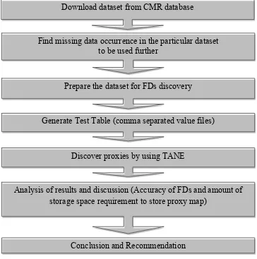
As shown in Figure 3.1, first step in this research is to check for the data available in the
Comprehensive Microbial Resources (CMR) and to download sample data sets. CMR is a
freely available website to show information about complete prokaryotic genome. As well,
this CMR database make easier by making availability of all the organisms information, it
also giving analysis of comparison between the genomes of the different organisms. CMR
also contains genome tools, searches for genes, genomes, sequence; comparative tool
which for comparison of multiple genomes. The tools could be more useful because it’s
providing graphical displays of genomes, biochemical pathways of genome as well. The
data were stored in a database called Omniome database. There are more than 20 tables in
data analysis in this research. In particular Taxon table has been selected in this research
since it has missing values in it.
And the second step is verifying presence of the missing values in the Taxon data
set. Taxan data set were viewed in Microsoft Office Excel and each column and row of the
table checked for missing values appearances. Statistic analysis was done on percentage of
missing data in taxon table. Step three is to prepare the dataset for FDs discovery. Datasets
must be separated into sub-tables and followed by reduction of missing data columns and
rows. Here the Taxon main table is spliced up into seven categories since it has 12
attributes. For ease of reference, attributes were presented as alphabets as shown in Table
2.
Table 2. List of attributes in Taxon
Attributes Represented by
U_id A
Taxon_id B
Kingdom C
Genus D
Species E
Strain F
Intermediate_rank_1 G
Intermediate_rank_2 H
Intermediate_rank_3 I
Intermediate_rank_4 J
Intermediate_rank_5 K
The first five column (attributes) A to E is remain unchanged for all the seven tables while
the balance seven attributes were spliced into seven table as follows: AE_F, AE_G, AE_H,
AE_I, AE_J, AE_K and AE_L. The attributes A, B C, D and E are never changed because
it has been found that those attributes does not have any missing values. Hence these
attributes remain the same to analyse the presence of FDs for the missing value analysis for
the other attributes. And the schemas of the sub-tables from Taxon are as follows:
i. AE_F = (A, B, C, D, E)
ii. AE_G = (A, B, C, D, G)
iii. AE_H = (A, B, C, D, H)
iv. AE_I = (A, B, C, D, I)
v. AE_J = (A, B, C, D, J)
vi. AE_K = (A, B, C, D, K)
vii.AE_L = (A, B, C, D, L)
Fourth step is to genere test table by data cleaning the taxon table into sub-table. After data
cleaning process, the data sets saved as comma separated values file to be used as input in
TANE. Sample input table data set is shown in Appendix A. Followed by step five, TANE
algorithm is used to detect the FDs in the test table which are generated before. TANE
algorithm was developed by Huhtala and colleageus. (Huhtala, et al., 1999). Step six will
be carried out experiment to obseve the missing values in test table and the original
complete table. Results from the experiment is used further for discussion of proxies for
space requirement analysis and aslo to recommend the characteristics of proxies for
Figure 7. Flow chart of overall methodology
3.3 Data source of Microbial Genomics data sets
As mentioned earlier in the methodology part, CMR database were chosen to get the
sample data set. Specifically microbial genomics database chose because most of the
diseases caused by the microbes called as pathogen. Hence there are many microbes has
been identified by the scientists in their research. Though, it is not properly managed to be
used in future; for example to obtain a vaccine or drug to cure a particular disease. Data
incompleteness may arise from this improper management of the database. Therefore,
sample data set were taken from CMR to analyse the presence of FDs which can be used in Download dataset from CMR database
Find missing data occurrence in the particular dataset to be used further
Prepare the dataset for FDs discovery
Generate Test Table (comma separated value files)
Discover proxies by using TANE
Analysis of results and discussion (Accuracy of FDs and amount of storage space requirement to store proxy map)
missing values prediction. Microbial genomics is the study of genome of microbes where it
determines the whole DNA sequence of the microbes. Along with this, the genes will
determine the functions and pathways of the microbes.
Chromosomes are made of nucleotides sequence which is called as gene that
encode specific product such RNA or protein molecule. Basically, gene contains biological
information for instance roles in cellular pathways and the location on a chromosome for
each specific species. The main characteristic of the genome is the taxonomic classification
(phylogenetic) including organism’s domains, phylum, class, order, family, genus, species
and strain. The reactions pathways are involving compounds such as reactants, and
enzymes to catalyse the reaction.
Fundamentally, genomics is the study of the organisation of genome’s molecule, its
content and the gene that they encode. It is divided into three categories such as structural
genomics, functional genomics, and comparative genomics. Structural genomics is the
study of the physical structure of an organism’s genomes. The major objective is to resolve
and explore the DNA sequence of the genome. Functional genomics is the analysis to
verify the genomes functions. The function is determined by the proteins that encode the
genome. The third category is comparative genomics to analyse the differences and
similarities in the genomes from different organisms. This analysis will help the
researchers to identify the conserved region in a particular genome and differentiate
function and regulation patterns.
DNA sequencing can be done using Sanger method. Whole-genome shotgun
sequencing is one of the simplest ways to analyse the microbial genomes. Here, fragments
of gene that has been produced were sequenced individually and computer is used to align
follows: library construction, random sequencing, fragment alignment and gap closure, and
editing.
Researchers have complete sequencing of many bacterial genomes and make
comparison between one another as well. This output will help us in identification and
determination of structure of genome, microbial physiology, phylogeny, and also the
pathogen that cause a disease. Identification of those criteria directly will help in producing
new vaccines and drugs for the disease treatment. At last, the function of genome can be
identified by annotation, where the DNA chips were used to study the mRNA synthesis
and the organism’s protein content. The extensive contribution of the genomes comparison
is the understanding of prokaryotic evolution and assists to assume the genes that are
responsible for different cellular processes.
3.2.1 Description of the semantics of Taxon table attributes
The taxon table holds the information about each genome filled into the omniome
database. Table db_data and taxon_link has linkage of genome information with taxon
table. Taxon table’s data was taken from NCBI. Taxon table has 14 attributes and 723 rows
of tuples. The attributes of Taxon table are:
Taxon = (u_id, taxon_id, kingdom, genus, species, comment, strain,
intermediate_rank_1, intermediate_rank_2, intermediate_rank_3,
intermediate_rank_4, intermediate_rank_5, intermediate_rank_6,
short_name)
Fundamentally, kingdom in biology is known as taxonomic rank which is the top
rank or three-domain system. Kingdoms are divided into three main domains such as
increase due to importance of molecular level comparisons of the genes is the key factor
besides genetic similarity and the physical appearance and behaviour.
In biology, genus (plural: genera) is the low-level taxonomic rank which is used to
classify the living and fossil organisms. Biodiversity studies especially fossil studies of a
species cannot always be identified and genera and families basically have lengthy ranges
than species which is determined by using genera and higher taxonomic level for instance
families.
Essentially species is a group of organisms that is capable of interbreeding and
reproducing good offspring. Normally species that shared common ancestors were placed
in one genus based on some similarities. The similarities are comparison of physical
attributes, for example their DNA sequences.
Strain also known as low-level taxonomic rank used in some of the biological field.
A strain is a genetic variant or a subtype of a micro-organism for instance virus, bacterium
or fungus. “Flu strain” is an example of the influenza or “flu” virus. Intermediate ranking
is about subdivision of the kingdom to get more specific gene for further use such as to
produce vaccine.
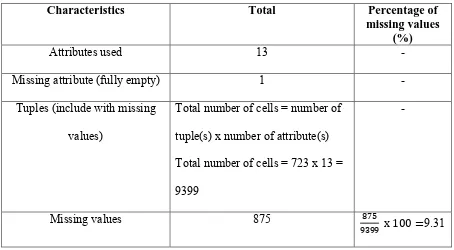
3.2.2 Observation of missing values in Taxon table
Out of 14 attributes 1 attribute (column: comment) is completely empty. There are
total 9399 tuples in the Taxon table. And 875 rows of tuples were missing in this table.
Statistics shows that about 9.31% data were missing. This missing data may cause some
problem during further analysis. For example loss of the specific gene or strain may cause
invariance results for organism classification. Statistics of the missing data is calculated
[image:34.595.78.532.175.425.2]based on the characteristics of Taxon table as shown in Table 3.
Table 3. Statistics of missing data in Taxon table
Characteristics Total Percentage of
missing values (%)
Attributes used 13 -
Missing attribute (fully empty) 1 -
Tuples (include with missing
values)
Total number of cells = number of
tuple(s) x numberof attribute(s)
Total number of cells = 723 x 13 =
9399
-
Missing values 875 875
9399 x 100 =9.31
3.4 TANE Algorithm for discovery of FDs
TANE is an available algorithm where presented by Huhtala et al. (1999) to discover FDs
that is not limited to small amount of datasets even for large number of datasets. This
algorithm is divided into few parts such as TANE main algorithm, generating levels,
computing dependencies, pruning the lattice, computing partitions, and approximate
dependencies. Fundamentally, TANE is partition based algorithm where set of rows are
partitioning their attributes which makes discovery of FDs faster and efficient. Besides
FDs, the partition also used to detect the AFDs with efficiently. “To find all valid minimal
manner”. (Huhtala, et al., 1999). The further details of the algorithm were explained in
section 3.3.1. Advantages of TANE are:
1. Fast even for a large number of tuples.
2. Not only FDs, discovery of approximate functional dependencies easy and efficient
and the erroneous or exceptional rows can be identified easily
3. Space can be pruned effectively and how the partitions and dependencies can be
computed efficiently.
The following are the steps involved in TANE algorithm process:
i. The installation of the data set must be done: For example the file (data set) name is
AE_F.orig. Save this file in “original” folder.
ii. Than open “description” folder and edit/create AE_F.dsc file to the variables.
iii. Create new data set by using select.perl command
% cd descriptions
%../bin/select.perl AE_F.dsc
(to produce AE_F.dat file in description folder)
iv. To get the output from the TANE: we use the following command
%bin/taneg3 <# of attributes> <# of records> <# of attributes> data/AE_F.dat 0.1 &>
TaxonAF01.txt
(the output file is in .txt format)
Huhtala et al., (1999) developed TANE algorithm for prediction of FDs. It is divided into
six subparts such as main TANE algorithm, generating levels, computing dependencies,
pruning the lattice, computing partitions, and approximate dependencies.
Figure 8shows the main TANE algorithm’s procedure. The computation in TANE
will begins with L1 = {{A} | A ϵ R} and work out L2 from L1 and L3 from L2. The step 6
COMPUTE_DEPENDENCIES (Lℓ) is to find the least dependencies with the left hand
side in Lℓ-1. Next the PRUNE (Lℓ) will search for the space. And then, the last step
GENERATE_NEXT_LEVEL (Lℓ) produces next level from the current level. (Huhtala, et
al., 1999).
Figure 8. TANE main algorithm (Adapted from Huhtala et al., 1999)
Figure 9 shows the subsequent algorithm from the main TANE algorithm; the
generating level algorithm. Here the GENERATE_NEXT_LEVEL is computing the Lℓ+1
from Lℓ. PREFIX_BLOCKS (Lℓ) is to sort the list of attributes with same prefix block.
Figure 9. Generating levels algorithm (Adapted from Huhtala et al., 1999)
After generating levels algorithm, COMPUTING_DEPENDENCIES is the next
step of TANE as in Figure 10. The output is to obtain minimal dependencies from this
procedure.(Huhtala, et al., 1999).
Figure 10. Computing dependencies algorithm (Adapted from Huhtala et al., 1999)
Procedure of pruning in TANE algorithm was given in Figure 11. Essentially, this
pruning procedure contains two parts; Rhs candidates pruning and key pruning. This
Figure 11. Pruning the lattice algorithm (Adapted from Huhtala et al., 1999)
The e value in TANE algorithm is calculated by stripped partitions procedure as in
Figure 12. An initialisation of table T to all NULL made through this procedure as an
assumption. The same table can be utilised repeatedly without re-initialisation because
before out the procedure resets to all NULL.
Figure 12. Computing partitions algorithm (Adapted from Huhtala et al., 1999)
The Figure 13 shows the approximate dependencies procedure. This procedure is
Beside this, it not only use to find the minimal approximate dependencies but with smaller
[image:39.595.84.539.118.340.2]error.
Figure 13. Approximate Dependencies algorithm (Adapted from Huhtala et al., 1999)
3.5 The method in preparing analysis of space requirement
Proxy based approach is designed for storage space optimisation. In this research, we adopt
proxy-based approach to study the requirement to predict missing values and types of
proxies which are contribute in save the space. Basically, the candidates proxies were
identified from the output produced from TANE algorithm, where the G3 errors are very
low or zero. If attribute shows very low or zero error, than it can be replaced to droppable
attribute to predict the missing values.
Pivot table can be used to count the number of instances in taxon proxy tables in
terms of space saving. Pivot table make it easy to arrange and summarise the complicated
data and drill down on details. Hence using this pivot table function in MS Excel, we
calculate the number of relationship between one tuple to another either one to one or one
3.5.1 Proxy based approach for space optimisation
The rising of data volumes in many application domains, makes raise a problem to
maintain such large data storages. Though, the storage space is reducible if the space of
storage was optimised. These space optimisations not only contribute to save the space, but
also decreasing the carbon footprint and the cost of operation. Beside this, it also
optimises query response time. Additionally, this space optimisation might make easy the
job of administering which are basically requires new infrastructure, utilities like power
and cooling increase, extra floor space and extra staff. (Emran, et al., 2012).
Therefore, Emran, Abdullah, and Isa (2012) produced an approach called
Proxy-based approach which can generate space optimisation through modification of database
schema. This can be done by deleting the attributes from the particular schema. The term
‘proxies’ were used by the researchers, is to replace the attribute with another attribute in
the schema. The functional dependency relationship is used to recognise the proxies among
the attributes in a relational table.
Basically, the space saving is obtained through some modification in the schema by
dropping some of the attributes. And then, the total saved space is approximately verified
by the number of attributes has been dropped and the tuples number in the table remain.
However, the droppable attribute and the proxy must have relationship in terms of missing
data. Hence, the functional dependency relationship is obtained between the attributes in
the relational tables. Proxies for the delete able attributes been found through discover of
the relations among attributes in the tables where there is presence of FD.
This proxy-based technique apply algorithm which will get back the removed
For instance, a and b are the droppable attribute. A proxy map consists of the following
mappings:
a → {1,2,3,4}, b → {5,6,7,8},
where the numbers are the proxy values and the arrow shows relationship mapping. From
here, the researchers have identified two types of proxy maps as follows:
i. A pure relational table:
This structure shows each value in a droppable attribute is matched to
exactly one value of the proxy. The schema structure of the table is:
<droppableAttr, proxy>. (Table 4)
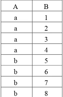
ii. A multi-valued table:
In this table, each value of droppable attribute is matched to a set of proxy
values. The schema structure of the table is: <droppableAttr, proxy>. (Table
[image:41.595.251.358.522.685.2]5)
Table 4. A Proxy map in pure relational table (Emran, Abdullah, and Isa 2012)
A B
a 1
a 2
a 3
a 4
b 5
b 6
b 7
b 8
A B a 1,2,3,4 b 5,6,7,8
The example also shows that, the size of proxy map in the multi-valued table is smaller
than the proxy map in pure relational table. As a result from the example, the storage space
can be saved by minimizing the proxy map in a multi-valued table structure as shown in
table 2.2. In the example above, the multi-valued table saves of 6 instances.
3.6 Conclusions
To conclude, the method has been applied according to research methodology described
above sections. The steps must be followed correctly to obtain precise results to be
analysed later. Results obtained from TANE algorithm saved as .txt file analysed and
discussed in the next chapter. The results were analysed according to accuracy or low G3
CHAPTER 4
RESULTS
4.1 Background
This chapter presents the results obtained from the steps performed in the methodology
which is described in the previous chapter. The input table used for this research is in
comma separated values file than saved as .txt file. The output also saved in the same
format to make easy to view the results. There are two types of results have been obtained
from the analysis:
i. Discovery of candidate proxies and its G3 values
ii. Amount of space required to store proxy information
4.2 Proxy discovery from Taxon sub-tables
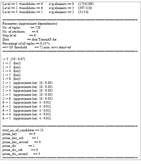
The TANE algorithm produced the output which can be viewed in notepad or WordPad.
Basically, the TANE algorithm has ten ranges which is start from 0.10 to 1.00. Since we
have total seven tables, each table can produce ten outputs. Figure 14 – Figure 23 show the
raw results for table AE_F produced by TANE algorithm and the other results were shown
in the Appendix B. Then, these results are analysed according to G3 ranges as described in
this sections above. Section 4.2.1 to 4.2.7 shows the summary of the output from TANE.
attribute that being analysed in each section. They are F, G, H, I, J, K, and L. This
identification is basically done according to the G3 errors values produced by the TANE
algorithm.
Level == 1 #candidates == 6 avg.elements == 8 (1710/208) Level == 2 #candidates == 6 avg.elements == 3 (397/118) Level == 3 #candidates == 1 avg.elements == 2 (31/14)
====================================================================== Parameters (approximate dependencies):
No. of tuples == 720 No. of attributes == 6 Stop level == 6
Data == data/TaxonAF.dat Percentage of all tuples == 0.10 %
==> G3 threshold == 72 max. rows removed
======================================================================
-> 3 (50 / 0.07) 1 -> 2 (key) 1 -> 3 (key) 1 -> 4 (key) 1 -> 5 (key) 1 -> 6 (key)
2 -> 1 (approximate key: 18 / 0.03) 2 -> 3 (approximate key: 18 / 0.03) 2 -> 4 (approximate key: 18 / 0.03) 2 -> 5 (approximate key: 18 / 0.03) 2 -> 6 (approximate key: 18 / 0.03) 6 -> 1 (approximate key: 4 / 0.01) 6 -> 2 (approximate key: 4 / 0.01) 6 -> 3 (approximate key: 4 / 0.01) 6 -> 4 (approximate key: 4 / 0.01) 6 -> 5 (approximate key: 4 / 0.01)
====================================================================== total_no_of_candidates == 13
prune_key == 9 prune_key_sub == 1 prune_key_second == 0 prune_rhs == 1 prune_rhs_sub == 0 prune_rhs_second == 3
[image:44.595.77.530.179.705.2]======================================================================
Level == 1 #candidates == 6 avg.elements == 8 (1710/208) Level == 2 #candidates == 6 avg.elements == 3 (397/118) Level == 3 #candidates == 1 avg.elements == 2 (31/14)
====================================================================== Parameters (approximate dependencies):
No. of tuples == 720 No. of attributes == 6 Stop level == 6
Data == data/TaxonAF.dat Percentage of all tuples == 0.20 %
==> G3 threshold == 144 max. rows removed
======================================================================
-> 3 (50 / 0.07) 1 -> 2 (key) 1 -> 3 (key) 1 -> 4 (key) 1 -> 5 (key) 1 -> 6 (key)
2 -> 1 (approximate key: 18 / 0.03) 2 -> 3 (approximate key: 18 / 0.03) 2 -> 4 (approximate key: 18 / 0.03) 2 -> 5 (approximate key: 18 / 0.03) 2 -> 6 (approximate key: 18 / 0.03) 6 -> 1 (approximate key: 4 / 0.01) 6 -> 2 (approximate key: 4 / 0.01) 6 -> 3 (approximate key: 4 / 0.01) 6 -> 4 (approximate key: 4 / 0.01) 6 -> 5 (approximate key: 4 / 0.01) 5 -> 4 (81 / 0.11)
====================================================================== total_no_of_candidates == 13
prune_key == 9 prune_key_sub == 1 prune_key_second == 0 prune_rhs == 2 prune_rhs_sub == 0 prune_rhs_second == 3
[image:45.595.77.528.75.622.2]======================================================================
Level == 1 #candidates == 6 avg.elements == 8 (1710/208) Level == 2 #candidates == 6 avg.elements == 3 (397/118) Level == 3 #candidates == 1 avg.elements == 2 (31/14)
====================================================================== Parameters (approximate dependencies):
No. of tuples == 720 No. of attributes == 6 Stop level == 6
Data == data/TaxonAF.dat Percentage of all tuples == 0.30 %
==> G3 threshold == 216 max. rows removed
======================================================================
-> 3 (50 / 0.07) 1 -> 2 (key) 1 -> 3 (key) 1 -> 4 (key) 1 -> 5 (key) 1 -> 6 (key)
2 -> 1 (approximate key: 18 / 0.03) 2 -> 3 (approximate key: 18 / 0.03) 2 -> 4 (approximate key: 18 / 0.03) 2 -> 5 (approximate key: 18 / 0.03) 2 -> 6 (approximate key: 18 / 0.03) 6 -> 1 (approximate key: 4 / 0.01) 6 -> 2 (approximate key: 4 / 0.01) 6 -> 3 (approximate key: 4 / 0.01) 6 -> 4 (approximate key: 4 / 0.01) 6 -> 5 (approximate key: 4 / 0.01) 5 -> 4 (81 / 0.11)
====================================================================== total_no_of_candidates == 13
prune_key == 9 prune_key_sub == 1 prune_key_second == 0 prune_rhs == 2 prune_rhs_sub == 0 prune_rhs_second == 3
[image:46.595.77.528.76.622.2]======================================================================
Level == 1 #candidates == 6 avg.elements == 8 (1710/208) Level == 2 #candidates == 6 avg.elements == 3 (397/118) Level == 3 #candidates == 1 avg.elements == 2 (31/14)
====================================================================== Parameters (approximate dependencies):
No. of tuples == 720 No. of attributes == 6 Stop level == 6
Data == data/TaxonAF.dat Percentage of all tuples == 0.40 %
==> G3 threshold == 288 max. rows removed
======================================================================
-> 3 (50 / 0.07) 1 -> 2 (key) 1 -> 3 (key) 1 -> 4 (key) 1 -> 5 (key) 1 -> 6 (key)
2 -> 1 (approximate key: 18 / 0.03) 2 -> 3 (approximate key: 18 / 0.03) 2 -> 4 (approximate key: 18 / 0.03) 2 -> 5 (approximate key: 18 / 0.03) 2 -> 6 (approximate key: 18 / 0.03) 6 -> 1 (approximate key: 4 / 0.01) 6 -> 2 (approximate key: 4 / 0.01) 6 -> 3 (approximate key: 4 / 0.01) 6 -> 4 (approximate key: 4 / 0.01) 6 -> 5 (approximate key: 4 / 0.01) 5 -> 4 (81 / 0.11)
====================================================================== total_no_of_candidates == 13
prune_key == 10 prune_key_sub == 1 prune_key_second == 0 prune_rhs == 2 prune_rhs_sub == 0 prune_rhs_second == 3
======================================================================
Level == 1 #candidates == 6 avg.elements == 8 (1710/208) Level == 2 #candidates == 6 avg.elements == 3 (397/118)
====================================================================== Parameters (approximate dependencies):
No. of tuples == 720 No. of attributes == 6 Stop level == 6
Data == data/TaxonAF.dat Percentage of all tuples == 0.50 %
==> G3 threshold == 360 max. rows removed
======================================================================
-> 3 (50 / 0.07) 1 -> 2 (key) 1 -> 3 (key) 1 -> 4 (key) 1 -> 5 (key) 1 -> 6 (key)
2 -> 1 (approximate key: 18 / 0.03) 2 -> 3 (approximate key: 18 / 0.03) 2 -> 4 (approximate key: 18 / 0.03) 2 -> 5 (approximate key: 18 / 0.03) 2 -> 6 (approximate key: 18 / 0.03) 5 -> 1 (approximate key: 300 / 0.42) 5 -> 2 (approximate key: 300 / 0.42) 5 -> 3 (approximate key: 300 / 0.42) 5 -> 4 (approximate key: 300 / 0.42) 5 -> 6 (approximate key: 300 / 0.42) 6 -> 1 (approximate key: 4 / 0.01) 6 -> 2 (approximate key: 4 / 0.01) 6 -> 3 (approximate key: 4 / 0.01) 6 -> 4 (approximate key: 4 / 0.01) 6 -> 5 (approximate key: 4 / 0.01) 4 -> 5 (322 / 0.45)
====================================================================== total_no_of_candidates == 12
prune_key == 10 prune_key_sub == 0 prune_key_second == 0 prune_rhs == 3 prune_rhs_sub == 0 prune_rhs_second == 3
[image:48.595.77.530.71.662.2]======================================================================
Level == 1 #candidates == 6 avg.elements == 8 (1710/208) Level == 2 #candidates == 6 avg.elements == 3 (397/118)
====================================================================== Parameters (approximate dependencies):
No. of tuples == 720 No. of attributes == 6 Stop level == 6
Data == data/TaxonAF.dat Percentage of all tuples == 0.60 %
==> G3 threshold == 432 max. rows removed
======================================================================
-> 3 (50 / 0.07) 1 -> 2 (key) 1 -> 3 (key) 1 -> 4 (key) 1 -> 5 (key) 1 -> 6 (key)
2 -> 1 (approximate key: 18 / 0.03) 2 -> 3 (approximate key: 18 / 0.03) 2 -> 4 (approximate key: 18 / 0.03) 2 -> 5 (approximate key: 18 / 0.03) 2 -> 6 (approximate key: 18 / 0.03) 5 -> 1 (approximate key: 300 / 0.42) 5 -> 2 (approximate key: 300 / 0.42) 5 -> 3 (approximate key: 300 / 0.42) 5 -> 4 (approximate key: 300 / 0.42) 5 -> 6 (approximate key: 300 / 0.42) 6 -> 1 (approximate key: 4 / 0.01) 6 -> 2 (approximate key: 4 / 0.01) 6 -> 3 (approximate key: 4 / 0.01) 6 -> 4 (approximate key: 4 / 0.01) 6 -> 5 (approximate key: 4 / 0.01) 4 -> 5 (322 / 0.45)
====================================================================== total_no_of_candidates == 12
prune_key == 10 prune_key_sub == 0 prune_key_second == 0 prune_rhs == 3 prune_rhs_sub == 0 prune_rhs_second == 3
[image:49.595.77.527.74.647.2]======================================================================
Level == 1 #candidates == 6 avg.elements == 8 (1710/208) Level == 2 #candidates == 6 avg.elements == 3 (397/118)
====================================================================== Parameters (approximate dependencies):
No. of tuples == 720 No. of attributes == 6 Stop level == 6
Data == data/TaxonAF.dat Percentage of all tuples == 0.70 %
==> G3 threshold == 503 max. rows removed
======================================================================
-> 3 (50 / 0.07) 1 -> 2 (key) 1 -> 3 (key) 1 -> 4 (key) 1 -> 5 (key) 1 -> 6 (key)
2 -> 1 (approximate key: 18 / 0.03) 2 -> 3 (approximate key: 18 / 0.03) 2 -> 4 (approximate key: 18 / 0.03) 2 -> 5 (approximate key: 18 / 0.03) 2 -> 6 (approximate key: 18 / 0.03) 4 -> 1 (approximate key: 463 / 0.64) 4 -> 2 (approximate key: 463 / 0.64) 4 -> 3 (approximate key: 463 / 0.64) 4 -> 5 (approximate key: 463 / 0.64) 4 -> 6 (approximate key: 463 / 0.64) 5 -> 1 (approximate key: 300 / 0.42) 5 -> 2 (approximate key: 300 / 0.42) 5 -> 3 (approximate key: 300 / 0.42) 5 -> 4 (approximate key: 300 / 0.42) 5 -> 6 (approximate key: 300 / 0.42) 6 -> 1 (approximate key: 4 / 0.01) 6 -> 2 (approximate key: 4 / 0.01) 6 -> 3 (approximate key: 4 / 0.01) 6 -> 4 (approximate key: 4 / 0.01) 6 -> 5 (approximate key: 4 / 0.01)
====================================================================== total_no_of_candidates == 12
prune_key == 11 prune_key_sub == 0 prune_key_second == 0 prune_rhs == 5 prune_rhs_sub == 0 prune_rhs_second == 1
[image:50.595.74.530.70.708.2]==================================================================
Level == 1 #candidates == 6 avg.elements == 8 (1710/208) Level == 2 #candidates == 6 avg.elements == 3 (397/118)
====================================================================== Parameters (approximate dependencies):
No. of tuples == 720 No. of attributes == 6 Stop level == 6
Data == data/TaxonAF.dat Percentage of all tuples == 0.80 %
==> G3 threshold == 576 max. rows removed
======================================================================
-> 3 (50 / 0.07) 1 -> 2 (key) 1 -> 3 (key) 1 -> 4 (key) 1 -> 5 (key) 1 -> 6 (key)
2 -> 1 (approximate key: 18 / 0.03) 2 -> 3 (approximate key: 18 / 0.03) 2 -> 4 (approximate key: 18 / 0.03) 2 -> 5 (approximate key: 18 / 0.03) 2 -> 6 (approximate key: 18 / 0.03) 4 -> 1 (approximate key: 463 / 0.64) 4 -> 2 (approximate key: 463 / 0.64) 4 -> 3 (approximate key: 463 / 0.64) 4 -> 5 (approximate key: 463 / 0.64) 4 -> 6 (approximate key: 463 / 0.64) 5 -> 1 (approximate key: 300 / 0.42) 5 -> 2 (approximate key: 300 / 0.42) 5 -> 3 (approximate key: 300 / 0.42) 5 -> 4 (approximate key: 300 / 0.42) 5 -> 6 (approximate key: 300 / 0.42) 6 -> 1 (approximate key: 4 / 0.01) 6 -> 2 (approximate key: 4 / 0.01) 6 -> 3 (approximate key: 4 / 0.01) 6 -> 4 (approximate key: 4 / 0.01) 6 -> 5 (approximate key: 4 / 0.01)
====================================================================== t