PI Controller Design Using Model Reference Adaptive Control Approaches For A Chemical Process.

PI Controller Design Using Model Reference

Adaptive Control Approaches

For A Chemical Process

M. R. Sapiee; F. Abdullah;A. Noordin;A. N. Jahari Faculty of Electrical Engineering, Universiti Teknologi Malaysia

Abstract—This paper discusses the application of Model Reference Adaptive Control (MRAC) concepts in designing an adaptive feedback controller to tune a given PI controller. The approaches of using the gradient (MIT) and stability (Lyapunov) methods are shown. The effectiveness of the two methods are shown through simulation and comparison is made to show which method give the best result. The results show that the stability method produces a better result.

Keywords — Model Reference Adaptive Control; gradient approach, MIT rule; stability approach, Lyapunov method

I. INTRODUCTION

In every day language “to adapt” means to change a behaviour to conform to new circumstances. At an early symposium in 1961 a long discussion ended with the following suggestion, an adaptive system is any physical system that has been designed with an adaptive viewpoint [1]. In this paper we deals with the pragmatic attitude to design a PI controller with adjustable parameters and a mechanism for adjusting the parameters by using the gradient approach (MIT) and the stability approach.

The aim of this assignment is to design two controllers for a chemical process based on the gradient and stability approaches. The performance of both will be compared via computer simulation to show the effectiveness of the controllers.

The paper is organized as follows. The MRAC theory of gradient method is presented in section III A and the stability approach is presented in section III B. The adaptive feedback controller scheme is presented in section IV. The simulation results are shown in section V. Finally, the results are concluded at the end of the paper.

II. PI CONTROLLER

An adaptive Proportional-Integral (PI) controller is required to control a chemical process. In PI-controller, there is another term in the controller equation [6].

( )

( )

( )

_⎟⎟

⎠ ⎞ ⎜

⎜ ⎝ ⎛

+

=

∫

t

I

dt t e T t e K t u

0 1

where TI is integration time constant. If the controller is tuned to be slow and TI is large, then the controller first acts

like P-controller, but later the as the integration starts to take effect, the steady-state deviation goes slowly to zero. In PI-control, the steady-state deviation will finally go to zero. If the controller is tuned to be fast and TI is small, then both terms (P and I) will affect the control signal all the way from the beginning. The system becomes faster, but the output signal might oscillates.

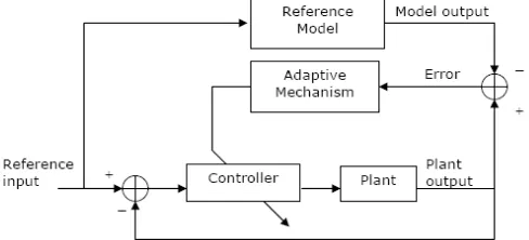
III. MODEL REFERENCE ADAPTIVE CONTROL Fig. 1 illustrates the general structure of the Model Reference Adaptive Control (MRAC) system. The basic MRAC system consists of 4 main components:

i) Plant to be controlled

ii) Reference model to generate desired closed loop output response

iii) Controller that is time-varying and whose coefficients are adjusted by adaptive mechanism

iv) Adaptive mechanism that uses ‘error’ (the difference between the plant and the desired model output) to produce controller coefficient

Regardless of the actual process parameters, adaptation in MRAC takes the form of adjustment of some or all of the controller coefficients so as to force the response of the resulting closed-loop control system to that of the reference model. Therefore, the actual parameter values of the controlled system do not really matter.

A. The Gradient Approach

The Gradient Approach/Method of designing an MRAC controller is also known as the MIT Rule as it was first

Figure 1. General structure of an MRAC system

Proceedings of 2008 Student Conference on Research and Development (SCOReD 2008),

26-27 Nov. 2008, Johor, Malaysia

978-1-4244-2869-4/08/$25.00 ©2008 IEEE

developed at the Massachusetts Institute of Technology (MIT), USA. This is the original method developed for adaptive control design before other methods were introduced to overcome some of its weaknesses. However, the Gradient method is relatively simple and easy to use.

In designing the MRAC controller, we would like the output of the closed-loop system (y) to follow the output of the reference model (ym). Therefore, we aim to minimise the error (e=y-ym) by designing a controller that has one or more adjustable parameters such that a certain cost function is minimised.

B. The Stability Approach

MRAC can be designed such that the globally asymptotic stability of the equilibrium point of the error difference equation is guaranteed. To do this, the Lyapunov Second Method is used. It requires an appropriate Lyapunov function to be chosen, which could be difficult. This approach has stability consideration in mind and is also known as the Lyapunov Method.

IV. ADAPTIVE FEEDBACK CONTROLLER DESIGN

The chemical process is described by the transfer functions and a controller by the form as indicated below where the time

delay TD and the time constant τ,of the process are unknown. Plant:

1 1

+ τ

= −

s e ) s (

G TDs ₍₁₎

Reference model:

1 5

1 +

= −

s e ) s (

G_m s (2) Controller:

) y r ( s k ky

u_{=− +} i _{− (3)}

A. Time Delay Approximation

A time delay element is represented by a non-linear transfer function. Since many control design methods require linear systems, it is often necessary to approximate a time delay by a linear transfer function [3,6]. Therefore, a suitable approximation is needed to represent the time delay term in the system.

There are many approximation methods available but for this assignment, we have selected Padé approximation. The Padé approximation for the time delay is given below:

2 2 +

+ − = −

s T

s T e

D D s

TD ₍₄₎

2 2 +

+ − = −

s s

e s (5) The above approximations will be used throughout this assignment in designing the controller.

B. The Gradient Approach Design

A closed-loop system with a controller that has the following parameters:

r(t) = Reference input signal u(t) = Control signal y(t) = Plant output

ym(t) = Reference model output

e(t) = Difference between plant and reference model output = y(t) - ym(t)

The control objective is to adjust the controller parameters, θ1 and θ2, so that e(t) is minimised. To do this, a cost function, J(θ) is chosen and minimised. Apart from Eqns. (1) through (5), the cost function chosen is of the form

2 2 1

e ) (

J θ = (6)

Let

s k_i

= θ₁ and

s k sk+ _i =

θ₂ . Replacing them into Eqn. (3), thus the controller, u becomes

y r

u=θ₁ −θ₂ (7) After time delay approximation using Eqns. (4) and (5), thus Eqns. (1) and (2), each becomes

Plant:

( )

(

2

)

2 2 2_{+ τ+ +} τ

+ − =

D D

D

T s

T

s T s

G (8)

Reference model:

( )

2 11 5

2 2_{+ +}

+ − =

s s

s s

G_m (9) Notice that from Eqn. (8),

(

T

)

s u s

T

s T y

D D

D _⋅

+ + τ + τ

+ − =

2 2

2

2 (10)

Then, after substituting Eqn. (7) into Eqns. (10),

(

)

(

)

(

)

2

2

1

2 2

2

2

θ + − + + + τ + τ

θ + − =

s T s

T s

T

r s T y

D D

D

D ₍₁₁₎

and from Eqn. (9),

(

)

2 11 5

2 2_{+ +}

+ − =

s s

r s

y_m

Therefore the error, e= y−y_m

(

)

(

)

(

)

(

)

2 11 5

2 2

2 2

2

2 2 2

1

+ +

+ − − + − + + + +

+ − =

s s

r s s

T s

T s

T

r s T e

D D

D

D

θ τ

τ

θ

So we have,

(

)

(

)

(

)

2

2 1

2 2

2

2

θ τ

τ γ θ

+ − + + + +

+ − ⋅

⋅ − =

s T s

T s

T

r s T e

dt d

D D

D

D

and

(

)

(

)

(

)

2

2 2

2 2

2

2

θ τ

τ γ θ

+ − + + + +

+ − ⋅

⋅ =

s T s

T s

T

y s T e

dt d

D D

D

D

In this case we need to do some approximation: i.e. perfect model following,y= ym. Therefore, we then have,

⎥⎦ ⎤ ⎢⎣ ⎡ + + + − ⋅ ⋅ ⋅ γ − = θ 2 11 5 2 2 1 s s s T r e dt d D s k s s s T r e s i D ₌ ⎥⎦ ⎤ ⎢⎣ ⎡ + + + − ⋅ ⋅ ⋅ − = 2 11 5 2 2 1

γ

θ

⎥⎦ ⎤ ⎢⎣ ⎡ + + + − ⋅ ⋅ ⋅ γ = θ 2 11 5 2 2 2 s s s T y e dt d _D s k k s s s T y e s i

D _{= +}

⎥⎦ ⎤ ⎢⎣ ⎡ + + + − ⋅ ⋅ ⋅ = 2 11 5 2 2 2

γ

θ

Which results in,

(

)

_⎢⎣⎡ _⎥⎦⎤ + + + − ⋅ + ⋅ ⋅ γ = 2 11 5 2 2 _s s s T y r e s

k D ₍₁₂₎

⎥⎦ ⎤ ⎢⎣ ⎡ + + + − ⋅ ⋅ ⋅ γ − = 2 11 5 2 2 s s s T r e s s

k_{i D}

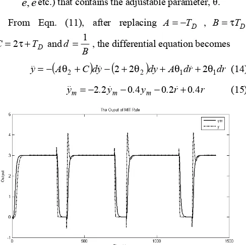
(13) The MRAC gradient approach is then simulated using Mathlab SIMULINK block with the reference input of a square wave signal with amplitude 3 and frequency 0.0033Hz. Both the output of the system responses (y and ym) are coupled and placed onto scope for simultaneous viewing. The scope is used to simultaneously observe the output response of y and the desired output response of ym.

Fig. 2 below shows the system output responses for a MIT rule based design with adaptation gains, gain1=0.02 and gain2=0.0015.

C. The Stability Approach Design

In designing an MRAC using Lyapunov Method, the following steps should be followed:

i) Derive a differential equation for error, e = y − ym (i.e.

e

,

e

etc.) that contains the adjustable parameter, θ.

From Eqn. (11), after replacing A=−T_D , B=τT_D

D

T

C=2τ+ and

B

d= 1 , the differential equation becomes

(

A C

)

dy

(

)

dy A dr dr y=− θ₂+ − 2+2θ₂ + θ₁ +2θ₁ (14)

r . r . y . y .

y_m=−22_m−04 _m−02+04 (15)

Figure 2. The outputs for y and ym for MRAC MIT Rules based design

Substituting Eqns. (14) and (15) into e=y−y_m, thus

dy d y Ad Ad A C e e

e 2.2 0.4 2 2.2 2 1 0.2⎟2

⎠ ⎞ ⎜ ⎝ ⎛ _{+ −} − ⎟ ⎠ ⎞ ⎜ ⎝ ⎛ _{+ −} − − − = θ θ dr d . r Ad Ad . 2 2 4 0 2 0 1 1 ⎟ ⎠ ⎞ ⎜ ⎝ ⎛_{θ −} + ⎟ ⎠ ⎞ ⎜ ⎝ ⎛ _+θ

+ (16)

ii) Find a suitable Lyapunov function, V(e,θ) - usually in a quadratic form (to ensure positive definiteness).

The Lyapunov function,V

(

e,e,X₁,X₂,X₃,X₄

)

, is based on

(16). 6 42

2 3 5 2 2 4 2 1 3 2 2 2

1e e X X X X

V=λ +λ +λ +λ +λ +λ

,

where 0 6 5 4 3 2

1 λ λ λ λ λ >

λ , , , , , is positive definite. The derivative of

V becomes

( )

(

)

(

)

(

5 3 1

)

3

(

6 4 1

)

4

2 1 2 4 1 1 1 3 1 2 2 1 2 2 2 2 2 2 2 4 . 0 4 . 4 X r e d X X r e Ad X X dy e X X y e Ad X e e e V λ λ λ λ λ λ λ λ λ λ λ + + + + − + − + − + − =

where for stabilityVmust be positive i.e. V<0.

iii) Derive an adaptation mechanism based on V(e,θ) such that e goes to zero.

2 3 2 1 5 2 θ = λ λ =

. Adey

X (17)

2 4 2 2 5 θ = λ λ =

dey

X (18) 1 5 2 3 5 2 θ = λ λ − =

. Ader

X (19)

1 6 2 4 5 θ = λ λ − =

der

X (20)

Summing Eqns. (17) and (18), results in

⎟⎟⎠ ⎞ ⎜⎜⎝ ⎛ λ λ + λ λ = θ 4 2 3 2 2 2 25

1. de Ay y

⎟⎟⎠ ⎞ ⎜⎜⎝ ⎛ λ λ ⎟⎟⎠ ⎞ ⎜⎜⎝ ⎛ λ λ + = + = θ 3 2 4 3 2 25 1

2 . Ad

ey A y e s k k i

Similarly, summing Eqns. (19) and (20) results in

(

)

⎟⎟⎠ ⎞ ⎜⎜⎝ ⎛ λ λ λ λ + λ λ − = θ 6 5 5 2 6 2 1 2 1 5 5

2. Ader der

⎟⎟⎠ ⎞ ⎜⎜⎝ ⎛ λ λ ⎟⎟⎠ ⎞ ⎜⎜⎝ ⎛ λ λ + − = = θ 5 2 6 5 1 25 1

2 . Ad

er a r e s k_i Therefore,

(

y y

)

e

(

r r

)

e

k=−γ₁ −4 −γ₂ −4

(

r r

)

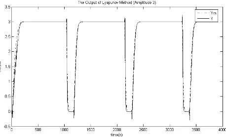
Fig. 3 below shows the outputs for y and ym for MRAC

Lyapunov Method based design with the adaptation gain value, 2

1 γ

γ & with 0.3 and 0.1 respectively. The output response of the system is displayed simultaneously in the scope similar to Fig. 1. The outputs for y and ym are stored in array in

MATLAB workspace for further analyses.

V. RESULTS COMPARISON AND DISCUSSION

The MRAC designed using the Gradient method/MIT rule has been shown that it does not guarantee stability to the resulting closed-loop system. On the other hand, designing an MRAC using the stability approach will ensure a stable closed loop system. Based on observation from the above designs, the differences of each design can be highlighted as below:

1. The adjustable parameter

θ

₁ and

θ

₂ for Lyapunov method are simpler than that of the MIT rule. The parameters of each adjustable design are summarized in Table 1.

TABLE I. ADJUSTABLEPARAMETERFORMRACDESIGN

Lyapunov Method MIT Rules

er dt

d

1 1 _{= −γ} θ

ey dt

d

2 2 _=γ θ

(

)

⎥⎦ ⎤ ⎢⎣

⎡

+ +

+ γ

= θ

2 11 5

2 2 1 1

s s

r As e dt d

(

)

⎥⎦ ⎤ ⎢⎣

⎡

+ +

+ γ

− = θ

2 11 5

2 2 2 2

s s

As y e dt

d

2. The performance of MRAC designs depend on the amplitude of the reference input signal, where the increase of amplitude from 1 to 3 will effect the above designs. It can be seen from Fig. 4 (a) and (b), that although the controllers designed based on both Gradient and Lyapunov Methods perform very well with r(t) of amplitude 1, when the amplitude of r(t) is changed to 3, the Gradient Method does not give very satisfactory results as the overshoots during transient is very high. This could result in the control actuator having to work extra hard at every cycle.

Figure 3. The outputs for y and ym for Lyapunov Method based design

Figure 4(a). The design outputs with reference signal amplitude of 1

Figure 4(b). The design outputs with reference signal amplitude of 3

VI. CONCLUSIONS

In conclusion, designing an adaptive controller through stability approach can ensure a stable closed loop system whereby the gradient approach does not take any consideration on the stability of the system. The stability approach produces a better result.

VII. ACKNOWLEDGEMENT

The authors would like to acknowledge their gratitude to Dr. Hazlina for her assistance in the completion of this paper. Not forgetting Sheikh Muhammad Hafiz Fahami, Alyaseh Nagi M Askir and Ahmed Mohamed Omran for their kind support.

REFERENCES

[1] G. Bartolini, "Adaptive and Sliding Mode Control', University of Cagliari, Cagliari, Italy, 2002

[2] Dr Hazlina Selamat, “Model Reference Adaptive Control (MRAC)” MEM1732 Lecture Notes, Malaysia: Universiti Teknologi Malaysia, 2008.

[3] K.Ogata, “Modern Control Engineering 4ed”, Prentice Hall 2002. pg 383.

[4] Z.K.Nagy, “SIMULINK for Process Control”, CG022/CGC047

Chemical Process Control Loughborough University 2008.

[5] M. Arcak, “Model Reference Adaptive Contol, ECSE/BMED 6480 – Adaptive Systems, University of California, 2001

[6] J. barraud et all, “PI Contollers Performances for a Process Model with Varying Delay, Institut Francais du Petrole.