Geographically Weighted Poisson Regression (GWPR) for Analyzing The Malnutrition Data (Case Study: Java Island in 2008

GEOGRAPHICALLY WEIGHTED POISSON REGRESSION (GWPR)

FOR ANALYZING THE MALNUTRITION DATA

(Case study: Java Island in 2008)

DIDIN SAEPUDIN

DEPARTMENT OF STATISTICS

FACULTY OF MATHEMATICS AND NATURAL SCIENCES

BOGOR AGRICULTURAL UNIVERSITY

2

ABSTRACT

DIDIN SAEPUDIN. Geographically Weighted Poisson Regression (GWPR) for Analyzing The Malnutrition Data (Case Study: Java Island in 2008). Advised by ASEP SAEFUDDIN and DIAN KUSUMANINGRUM.

Poisson regression, namely global model is a statistical method used to analyze the relationship between the dependent variable and the explanatory variables, where the dependent variable is a counted data and has a Poisson distribution. The result of its parameter estimation is homogeneous for all of the observations. However, especially in spatial data, its estimation will produce biased estimation. The parameter estimates in each location will vary among regions as it is influenced by territorial or geographical factors, which is known as spatial variability or spatial non-stationarity. Therefore the appropriate analysis for this data is Geographically Weighted Poisson Regression (GWPR) model. GWPR parameter estimation used a weighting matrix which depends on the proximity between the locations. Fisher scoring iteration is used for solving the iteratively parameter estimation. In this research, GWPR will be used in malnutrition data because malnutrition is counted data which is assumed to have a Poisson distribution and the indirect factors of differences in the number of malnourished patients in every region is possible due to spatial factors. The results showed that GWPR model has better performance than global model based on AICc difference. Poverty aspect was the most influencing factor to the number of malnourished patients in a region compared to health, education, and food aspect. The spatial variability map is created for eight variables used in selected global model where every map showed the variability of local parameter estimates. There were five groups of the local parameter estimates in each map based on percentiles grouping which showed the low until hight relation of the parameter estimates groups to the number of malnourished patients. This research also created a significant variables map which detects the variables that were significant in each region. Keywords: spatial non-stationarity, Geographically Weighted Poisson Regression (GWPR),

GEOGRAPHICALLY WEIGHTED POISSON REGRESSION (GWPR)

FOR ANALYZING THE MALNUTRITION DATA

(Case study: Java Island in 2008)

DIDIN SAEPUDIN

Scientific Paper

to complete the requirement for graduation of Bachelor Degree in Statistics at Department of Statistics

Faculty of Mathematics and Natural Sciences Bogor Agricultural University

DEPARTMENT OF STATISTICS

FACULTY OF MATHEMATICS AND NATURAL SCIENCES

BOGOR AGRICULTURAL UNIVERSITY

4

Title : GEOGRAPHICALLY WEIGHTED POISSON REGRESSION (GWPR) FOR ANALYZING THE MALNUTRITION DATA (Case study: Java Island in 2008) Name : Didin Saepudin

NRP : G14080012

Approved by,

Advisor I Advisor II

Dr. Ir. Asep Saefuddin, M.Sc NIP. 19570316 198103 1 004

Dian Kusumaningrum, M.Si.

Acknowledged by, Head of Department of Statistics Faculty of Mathematics and Natural Sciences

Bogor Agricultural University

Dr. Ir. Hari Wijayanto, M.Si NIP. 19650421 1999002 1 001

ACKNOWLEDGEMENTS

Alhamdulillahi rabbil ‘alamin, praise be to Allah SWT, God of the universe. The author felt deeply grateful to Allah SWT for all the blessing and guidance that made this paper entitled “Geographically Weighted Poisson Regression (GWPR) for Analyzing The Malnutrition Data (Case Study: Java Island in 2008)”.

The author realizes that the completion of this research would not be possible without the support and help from many people. The author would like to express his sincere gratitude to the advisors, Mr. Asep Saefuddin and Mrs. Dian Kusumaningrum for his/her guidance and suggestion for this research and also to Mr. Tomoki Nakaya, Professor of Geography Department in Ritsumeikan University, for the enlightening discussion and giving the GWPR references by e-mail. The author is also grateful to his beloved family for their never ending prayer, love, and support, especially to his mother, alm. Warti for her forever lasting love. Gratitude is shown to all of his friends in Statistika 45, Sylvasari Dormitory, and Sylvapinus Dormitory for their empatiness, spirit, and togetherness in finding knowledge. Gratitude is also to Rama, Liara, and Dania as Mr. Asep Saefuddin’s advised friends for giving the spirit and support in his research. Hopefully, this paper would be useful for all.

Bogor, December 2012

6

BIOGRAPHY

The author was born in Cilacap, October 13th, 1989 as the son of Nono Darsono and alm. Warti. He is the first son with two brothers. The author graduated from MIN 1 Dayeuhluhur in 2002 and from SMPN 1 Dayeuhluhur in 2005. By the year 2008, he graduated from SMAN 1 Dayeuhluhur and at the same year, he enrolled in Bogor Agricultural University through USMI (Undangan Seleksi Masuk IPB) as a student of Department of Statistics, Faculty of Mathematics and Natural Sciences and took Actuarial and Finance Mathematics as a minor programme.

CONTENTS

Page

LIST OF FIGURE ... viii

LIST OF TABLE ... viii

LIST OF APPENDIX ... viii

INTRODUCTION ... 1

Background ... 1

Objectives ... 1

LITERATURE REVIEW ... 1

Definition of Malnutrition ... 1

Poisson Regression Model ... 2

Breusch-Pagan (BP) test ... 2

Geographically Weighted Regression (GWR) ... 2

Parameters Non-stationarity ... 3

Geographically Weighted Poisson Regression (GWPR) ... 3

Standard Error of Parameters in GWPR ... 4

Parameters Significance Test in GWPR ... 4

Kernel Weighting Function ... 4

Akaike Information Criterion ... 4

METHODOLOGY ... 5

Data Sources ... 5

Methods ... 5

RESULT AND DISCUSSION ... 5

Data Exploration ... 5

Variables Selection ... 6

Global Model ... 6

Spatial Variability Test ... 6

Parameters Estimate Interpretation of Global Model ... 7

Bandwidth Selection ... 8

GWPR Model ... 8

Stationary Parameter and Fitted Model of GWPR ... 8

Spatial Variability Map ... 9

Significant Explanatory Variables Map ... 12

CONCLUSION AND RECOMMENDATION ... 13

Conclusion ... 13

Recommendation ... 13

8

LIST OF FIGURE

Page

Figure 1 Stationary versus non-stationary based on concept from Fotheringham et al. (2002) .. 3

Figure 2 Effective number of GWPR parameters (K) and the AICc plotted against adaptive kernel bandwith ... 8

Figure 3 Absolute residual of GWPR and global model plotted against observations ... 8

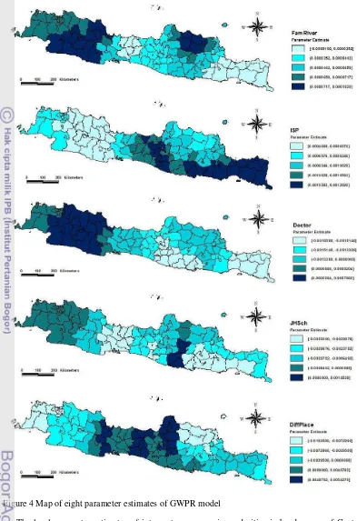
Figure 4 Map of eight parameter estimates of GWPR model ... 9-10 Figure 5 Significant Explanatory Variables Map ... 12

LIST OF TABLE

Page Table 1 Parameter estimate and p-value of t-test of global model with seven explanatory variables ... 6

Table 2 Comparison of AICc value between two global models ... 6

Table 3 Breusch-Pagan test statistics ... 7

Table 4 Comparison of AICc value beetwen global model and GWPR model ... 8

Table 5 Simple test for non-stationary parameter estimate ... 9

LIST OF APPENDIX

Page Appendix 1 Description of dependent variable and explanatory variables ... 15

Appendix 2 Algorithm of research method ... 16

Appendix 3 Map of malnourished patiens distribution for each regency and city in Java island (2008) ... 17

Appendix 4 Boxplot of dependent variable and explanatory variables ... 18

Appendix 5 Pearson’s correlation between variables (dependent variable and explanatory variables) ... 19

INTRODUCTION

Background

Poisson regression is a statistical method used to analyze the relationship between the dependent variable and the explanatory variables, where the dependent variable is in the form of counted data that has a Poisson distribution. For example, the case of relation between cervical cancer disease incidence rates in England and socio-economic deprivation (Cheng et al. 2011). In the parameter estimation, it is assumed that the fitted value for all of the observations or regression points are the same. This assumption is referred to as homogeneity (Charlton & Fotheringham 2009).

However, there is a problem if the observations are recorded in a regional or territorial data, which is known as spatial data. If the spatial data was analyzed by Poisson regression, it will ignore the variation across the study region. The decision to ignore potential local spatial variation in parameters can lead to biased results (Cheng et al. 2011). Whereas, the local spatial variation can be important and such information may have important implications for policy makers.

In the case of spatial processes which is referred to spatial non-stationarity (Fotheringham et al. 2002). Geographically Weighted Poisson Regression (GWPR) will be the most appropriate analysis if the data has a non-stationary condition and the dependent variable was assumed Poissonly distributed. GWPR model uses weighting matrix which depends on the proximity between the location of the observation. In this research, a modified local Fisher scoring procedure is used to estimate the local parameters of GWPR iteratively and using the bi-square adaptive Kernel function to find the weighting matrix is expected. The Kernel function determines weighting matrix based on window width (bandwidth) where the value is accordance with the conditions of the data and adaptive because it has a wide window (bandwidth) that varies according to conditions of observation points.

Malnutrition data in Java island was choosen in this research because the number of malnourished patients was counted data which was assumed to have a Poisson distribution. Based on the data taken from National Institute of Health Research and Development (2008), there are differences of malnutrition prevalence in every province in Java island. The malnutrition prevalence was

based on indicators of Weight/Age (BB/U), East Java (4.8%) had the highest malnutrition prevalence, followed by Banten (4.4%), Central Java (4.0%), West Java (3.7%), DKI Jakarta (2.9%), and Jogjakarta (2.4%). These difference can be related to the phenomenon of spatial variability. The variability of malnutrition prevalence in each province might vary in each city or regency. Directorate of Public Health Nutrition (2008) described that the indirect factors that influence malnutrition are food supply, sanitation, health services, family purchasing power and the level of education. Nevertheless geographical aspect could also influence malnutrition. Handling the malnutrition case is very important because malnutrition will directly or indirectly reduce the level of children intelligence, impaired growth and children development and decreased the productivity.

The research that analyzed the affected factors that affect malnutrition which is also associated with spatial effect has been carried out by several researchers. Two researchers who have analyzed it were Rohimah (2011) with the title of thesis “Spatial Autoregressive Poisson model for Detecting the Influential Factors of the number of Malnourished patients in East Java” and A’yunin (2011) who analyzed “Modeling of Malnutrition Infants Under Five (Toddlers) in Surabaya with Spatial Autoregressive Model (SAR)”. However, there was only one of the research, which is related with Geographically Weighted Poisson Regression (GWPR), was analyzed by Aulele (2010) in his thesis entitled “Geographically Weighted Poisson Regression Model (Case Study: The Number of Infant Mortality in East Java and Central Java 2007)”. The difference of this research with the previous research is the researcher has created a local model for each regency or city in Java island. The researcher also created a spatial variability map for making it more easy to interprete the local parameter estimates.

Objectives

The objectives of this research are:

1. To compare the better model between global Poisson model and GWPR model for the malnutrition data in Java

2. To create the spatial variability map 3. To analyze the factors influencing the

2

LITERATURE REVIEW

Definition of Malnutrition

Based on Statistics Indonesia (2008), definition of malnutrition is a condition of less severe level of nutrients caused by low consumption of energy and protein in a long time characterized by the incompatibility of body weight with age. Directorate of Public Health Nutrition (2008) described that malnutrition is directly caused by the lack of food intake and infectious diseases and it is indirectly caused by the availability of food, sanitation, health care, parenting, family purchasing power, education and knowledge.

Poisson Regression Model

The standard model for counted data is the Poisson regression model, which is a nonlinear regression model. This regression model is derived from the Poisson distribution by allowing the intensity parameter

μ

to depend on explanatory variables (Cameron & Trivedi 1998).

Probability to count the numbers of events yi (dependent variable for ith observation) given variable x can be defined as:

Pr(yi|x_i) =

where,

yi = 0,1,2,...

i = 1,2,...,n

μi = E(yi|x_i)=exp( ) x_i

= [1,x_i1,...,xik]

k = the number of explanatory variables (Long 1997).

Fleiss et al. (2003) has defined the Poisson regression model as,

ln μi = β0 + β1xi1 + β2xi2 + ... + β(p-1)xi(p-1) = , where p is the number of parameters regression. μi is the expected value of Poisson distribution for observation ith and

β = [ β0,β1,..., βp-1]. The factor change in the expected count for a change of in xk equals,

Therefore, the parameter can be interpreted as for a change of in xk, expected count increase by a factor of , while all

other variables are considered constant (Long 1997).

Breusch-Pagan Test (BP-test) Breusch and Pagan (1979) in Arbia (2006) proposed a generic form of homoscedasticity expressed by the following equation,

is a set of constants. is the constant term of the regression and are the constant terms for the regressors. The null and alternative hypothesis of BP-test are:

H0 :

H

1

:

i

, where

; (

i

=2,3,...,k)

Under H0, we assume that = constant. Spatial variability is simply structural instability in the form of non-constant error variances (heteroscedasticity) or model coefficients (variable coefficients, spatial regimes) and can be tackled by means of the standard econometric toolbox. One of the reasons why it is important to consider spatial variability, explicitly the “structure” of data behind the instability is spatial (or geographic) in the sense that the location of the observations is crucial in determining the form of the instability. For example, groupwise heteroscedasticity could be modeled as different error variances for different compact geographic subsets of the data (Anselin 1999).

Anselin (1988) in Arbia (2006) has described that Breusch-Pagan test statistics can be derived using the general expression of the Lagrange multiplier test, which could be expressed as:

1 1 1

1

( ) '( ')( )

2   





n i i



n i i



n i i

i i i

BP x f x x x f (1)

where, ̂ _̂ ̂ ̂ ̂ ∑ ̂

The test-statistic in equation (1) has a χ² distribution with k-1 degrees of freedom (k is the number of explanatory variables).

0

1

( , ) ( , ) p

i i i k i i ik i

k

y



u v



u v x





 





where {β0(ui,vi),...,βk(ui,vi)} are k+1 continuous functions of the location (ui,vi) in the geographical study area. The εis are random error terms (Fotheringham et al. 2002).

Parameters Non-stationarity Fotheringham et al. (2002) has described that the data is in a stationary condition if the data is homogenous across the study region, otherwise it is known to be non-stationary. In the non-stationary condition, it investigates that the parameter estimates might not be constant over space. Clearly, any relationship that is non-stationary over space will not be well-represented by a global statistic and this global value may be misleading locally. It is therefore useful to conduct an indepth study on why relationships might vary over space. If there is no reasonable suspect that the parameters vary, there is no need to develop local statistical methods.

Figure 1 ` Stationary versus non-stationary based on concept from Fotheringham et al. (2002)

Geographically Weighted Poisson Regression

Geographically Weighted Poisson Regression (GWPR) model is a developed model of GWR where it brings the framework of a simple regression model into a weighted regression. Coefficients of GWPR can be estimated by calibrating a Poisson regression model where the likelihood is geographically weighted, with the weights being a Kernel function centred on u_i (u_i is a vector of location coordinates (ui,vi)) (Nakaya et al. 2005).

The steps used to estimate the coefficients of GWPR are:

1. Make a likelihood function of Poisson distribution from the n-numbers of response variable (yi~Poisson (μ(x_i,β)):

L(β) =

1

n

i



( ) (2)

where μ = exp( ) (Long 1997).

2. Maximize the log-likelihood function in equation (2):

lnL( )=

n

i = 1



( i )+

n

i = 1



(x_i

n

i = 1



(Fleiss et al. 2003)

3. Fotheringham et al. (2002) has described that an observation in GWPR is weighted in accordance with its proximity to location ith. So, the equation in the 2nd step can be expressed as:

ln*L( ui,vi))={

n

i = 1



( _i ui,vi))+

n

i = 1



yi(x_i (u_i,vi))

n

i = 1



}wij(ui,vi) 4. Make a partial derivatives of equation

above with respect to the parameters in (ui,vi) and its result must be equal to zero:

={

n

i = 1



i ( i ui,vi))+

n

i = 1



x_i y_i}w_ij(u_i,vi) = 0 (3)

However, this equation is iterative.

5. Based on Nakaya et al. (2005), The maximization problem in the equation (3) can be solved by a modified local Fisher scoring procedure, a form of Iteratively Reweighted Least Squares (IRLS). The iterative procedure is necessary except for the special case of Kernel mapping. In this local scoring procedure, the following matrix computation of weighted least squares should be repeated to update parameter estimates until they converge:

_{(ui,vi) = (X'W(ui,vi)A(ui,vi)}(l) X)-1 X'W(ui,vi)A(ui,vi)(l)z(ui,vi)(l) where is a vector of local parameter estimates specific to location i and superscript (l+1) indicates the number of iterations. The vector of local parameter estimates specific to location i when lth iteration is defined as:

_{(ui,vi) = (}

4

X is a design matrix and X' denotes the transpose of X.

( ₎

W(ui,vi) denotes the diagonal spatial weights matrix for ith location:

W(ui,vi) = diag[wi1, wi2,..., win]

and A(ui,vi)(l) denotes the variance weights matrix associated with the Fisher scoring for each ith location:

A(ui,vi)(l) = diag [ ̂ ( (ui,vi)), ̂ ( (ui,vi)),..., ̂ ( (ui,vi))]

Finally, z(ui)(l) is a vector of adjusted dependent variables defined as:

z(l)(ui,vi)=[z1(l)(ui,vi),z2(l)(ui,vi),..., zn(l)(ui,vi)]' By repeating the iterative procedure for every regression point i, sets of local parameter estimates are obtained.

6. At convergence, we can omit the subscripts (l) or (l+1) and then rewrite the estimation of (ui,vi) as:

̂(ui,vi) = (X'W(ui,vi)A(ui,vi)X)-1X'W(ui,vi) A(ui,vi)z(ui,vi)

Standard Error of Parameters in GWPR The standard error of the kth parameter estimate is given by

Se( k(ui,vi)) =√ ̂ where,

cov( ̂(ui,vi)) = C(ui,vi)A(ui,vi)-1[C(ui,vi)]' C(ui,vi) = X'W(ui,vi)A(ui,vi)X)-1

X'W(ui,vi)A(ui,vi).

cov( ̂(ui,vi)) is the variance–covariance matrix of regression parameters estimate and ̂ is the kth diagonal element of cov( ̂(ui,vi)) (Nakaya et al. 2005).

Parameters Significance Test in GWPR Hypothesis for testing the Significance for the local version of the kth parameter estimate is described as:

H0 : k(ui,vi) = 0

H1 : k, where k(ui,vi) 0 ; (k=0,1,2...,(p-1)).

The local pseudo t-statistic for the local version of the kth parameter estimate is then computed by:

k(ui,vi) =

This can be used for local inspection of parameter significance. The usual threshold of p-values for a significance test is effectively |t|>1.96 for tests at the five percent level with large samples (Nakaya et al. 2005).

Kernel Weighting Function

The parameter estimates at any regression point are dependent not only on the data but also on the Kernel chosen and the bandwidth for that Kernel. Two types of Kernel that can be selected are a fixed Kernel and an adaptive Kernel. The adaptive Kernel permits using a variable bandwidth. Where the regression points are widely spaced. The bandwidth is greater when the regression points are more closely spaced (Fotheringham et al. 2002).

The particular function in adaptive Kernel’s method is a bi-square function. A bi-square function where the weight of the jth data point at regression point i is given by:

2 2

( ) ( )

( )

[1 ( / ) ] ; when

0 ; when

ij i k ij i k

ij

ij i k

d b d b

w d b       _ 

where wij is weight value of observation at the location j for estimating coefficient at the location i. dij is the Euclidean distance between the regression point i and the data point j and bi(k) is an adaptive bandwidth size defined as kth nearest neighbour distance (Fotheringham et al. 2002).

Akaike Information Criterion The Akaike Information Criterion (AIC) of the model with bandwidth b is defined as:

AIC(b) = D(b) + 2K(b)

where D and K denote the deviance and the efective number of parameters in the model with bandwidth b respectively (Fotheringham et al. 2002). The deviance of Poisson regression model is defined as:

1

ˆ

2

ln

(

)

ˆ















































n i

i i i

i i

y

D

y

y

called MAICE (minimum AIC estimator) (Fotheringham et al. 2002).

Sugiura (1978) in Burnham & Anderson (2002) derived a second-order variant of AIC that he called AICc (corrected Akaike Information Criterion). Formula of AICc is:

AICc(b) = AIC(b) + If sample sizes is large with respect to the number of estimated parameters or when the ratio n/K is small (say < 40), using AICc is recommended (Burnham & Anderson 2002). But, If the ratio n/K is sufficiently large, then AIC and AICc are similar and will strongly tend to select the same model. A common rule-of-thumb in the use of AICc is that if the difference in AICc values between two models is less than or equal to 2, then two models are as good as model. Otherwise, the difference in AICc values between two models is greater than to 2, there is significant difference between the two models and the minimum AICc as a good model (Nakaya 2005). Fotheringham et al. (2005) have described that AIC and AICc also can be used to select the optimal bandwith with the minimum AIC or AICc.

METHODOLOGY

Data Sources

The data used in this study are secondary data from Potensi Desa (Podes) data in 2008. The objects of this research are 112 regrencies and cities in Java island.

The dependent variable used in this research is the number of malnourished patients in each regency and city in Java island. The explanatory variables is selected from four aspects, which include poverty, health, education, and food aspect. There were 14 explanatory variables used which is described in detail in Appendix 1.

Methods

The methods used in this research are: 1. Explore the data

2. Check the multicolinearity among the explanatory variables by using the Pearson’s correlation

3. Make a best model for global Poisson regression model, namely global model with the folowing steps:

a) Modeling with all of selected explanatory variables from previous step

b) Select the explanatory variables which were significant to the dependent variable (with p-value of parameter estimates are equal to or lower than five percent and 15 percent)

c) Make a global model from combinations of selected explanatory variables

d) Compare the AICc value among the models created

e) Select the best model (with criteria of AICc difference is less than 2)

4. Test the spatial variability of the data by Breusch-Pagan test

5. Interpretation of parameter estimate in global model

6. Analyze a local model of GWPR, by using the folowing steps:

a) Determine the value of longitude and latitude (ui,vi) for every regency and city in Java island

b) Determine the optimum bandwidth by the minimum AICc

c) Calculate the weighted matrix by the bi-square adaptive Kernel function for each regency or city

d) Estimate the parameter of GWPR with a modified local Fisher scoring procedure for solving the parameter estimate iteratively

e) Test the spatial non-stationary f) Create a fitted model of GWPR 7. Test the goodness of fit between global

model and GWPR model by the minimum AICc estimation (with criterion of AICc difference is less than 2)

8. Interpretation of the GWPR parameters 9. Create a map of spatial variability for each

parameters of GWPR

10.Interpretation of the spatial variability map.

The algorithm of research method can be seen in Appendix 2. The Softwares that was applied for this research are GWR 4.0, R 2.15.0, and ArcGIS 3.2.

RESULT AND DISCUSSION

Data Exploration

6

malnourished patients in the regions of DKI Jakarta province are low which is lower than 500 patiens. The regions with high numbers of malnourished patiens must be handled seriously than the others. One of the solution is by determining the infulencing factors to the malnourished patiens for each regions. If the factors have been known, it can be used by policy maker for solving this problem.

A boxplot was also used for exploring the data. The figure of boxplot for each variable was shown in Appendix 4. From the boxplot, it can be seen that there were five explanatory variables that does not have outliers, which were FamLabour, Illiteracy, ISP, ActISP, and HlthWrk variable. The other explanatory variables have upper extreme values as outliers. The outliers were found in the regions with high values of FamLabour, Illiteracy, ISP, ActISP, and HlthWrk. As for an example, Bogor regency have upper extreme value in FamSlums, JHSch, and ElmSch variable. It means that Bogor regency have high number values of families residing in the slums, and many of their people hare junior high schools or equivalent, or elementary schools or equivalent education. Therefore the outliers in each of the variables are still used in further analysis because every region will be created a local model of GWPR.

Variables Selection

Variable selection in developing the GWPR model is done by exploring the correlation between two explanatory variables using Pearson’s correlation, which is showed in Appendix 5. The explanatory variable with higher correlation to dependent variable (if there are two variables that are highly correlated) is choosen for the global model. From 14 explanatory variables, there are only seven explanatory variables that are not highly correlated to each other. They were FamLabour, FamRiver, FamSlums, ISP, Doctor, DiffPlace, and JHSch variable. Therefore, these seven variables were used in the further analysis. All of the aspects are represented in the selected explanatory variables.

Global Model

A traditional global Poisson regression model, namely global model, was fitted to the malnourished patients in one regency or city based on the selected explanatory variables. As explained above, seven explanatory variables were selected and used to create

global model. Their parameter estimates and p-values are displayed in Table 1.

Table 1 Parameter estimates and p-values of t -tests of global model with seven explanatory variables

Covariate Estimate Pr(>|t|) Intercept 5.039338 < 2x10-16* FamLabour 0.000002 < 2x10-16* FamRiver 0.000053 < 2x10-16* FamSlums -0.000008 < 1.46x10-12* ISP 0.00074 < 2x10-16*

Doctor -0.000029 0.124

DiffPlace 0.001539 < 7.74x10-9* JHSch -0.001113 < 2x10-16* *significant at = 5%

A Global model from seven explanatory variables, namely global model 1, showed that only one variable was not significant at five percent level of significance which was Doctor variable. Therefore another global model candidate will be created without using Doctor variable, namely global model 2. Global model 2 resulted that all of variables were significant. But, we can not select directly that global model 2 was the best model. To compare it with global model 1, the difference of AICc values was used as a criterion to select the best model.

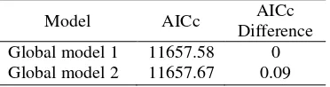
Table 2 Comparison of AICc value between two global models

Model AICc AICc

Difference Global model 1 11657.58 0 Global model 2 11657.67 0.09

Based on the criterion of selecting the best model with the AICc difference between two models is less than or equal to 2 (Nakaya et al. 2005). Both models are considered as a good model because the AICc difference is lower than 2. But, global model 1 will be selected as best model to create GWPR model because its AICc difference is very small and this model accomodated all factors. Therefore, it will explain the influencing factors of the number of malnourished patients better.

Spatial Variability Test

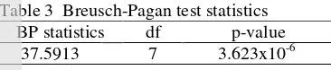
Table 3 Breusch-Pagan test statistics BP statistics df p-value

37.5913 7 3.623x10-6 From Table 3, the p-value of BP test was significant at a five percent significance level. It means that there are variability among observations. Therefore, there are special characteristics for each region. Hence, the data must be analyzed by local modeling in order to capture the variation of data and explain the characteristic of each region better.

Parameters Estimate Interpretation of Global Model

In the previous discussion, the global model used for developing the next modeling is global model 1. The selected explanatory variables were FamLabour, FamRiver, FamSlums, ISP, Doctor, DiffPlace, and JHSch variable. The final fitted global model is:

ln ̂ = 5.039338 + 0.000002 FamLabour + 0.000053 FamRiver

- 0.000008 FamSlums

+ 0.000740 ISP- 0.000029 Doctor + 0.001539 DiffPlace - 0.001113

JHSch (4)

From equation (4), all of the aspects are represented in the final fitted global model. The aspect of poverty is represented by FamLabour, FamRiver, and FamSlums variable. The health aspect are represented by ISP and Doctor variable. Education and food aspect is represented only by JHSch variable as an education aspect and DiffPlace variable as a food aspect.

In the poverty aspect, FamLabour and FamRiver variables are positively related, but FamSlums variable is negatively related to the number of malnourished patients in a region. Actually, poverty affects health, so the poor people are vulnerable to various kinds of diseases, one of them is malnutrition (http://www.ppjk.depkes.go.id/index.php?opti on=com_content&task=view&id=53&Itemid= 89). In this case, FamLabour and FamRiver variable was enough to explain the positive relation of poverty aspect with the number of malnourished patients. It means that the regions with high counts of poor people would have high counts of malnourished patients. In the parameter interpretation, the parameter estiamate of FamLabour was used for an example. With the Increasing of 1000 family whose members are farm labour, the expected number of malnourished patients will increase around 1,000 persons in each regency or city

(assuming that all of other parameter estimates are constant).

Next, the health aspect represented by ISP and Doctor variables. Relation of ISP and Doctor variables to the number of malnourished patients are different. The ISP variable is positively related, but the Doctor variable is negatively related. In expectation, the better organizing of health aspect in a region, will cause the number of malnourished patients to decrease. One of the reason that the ISP variable has a positive parameter estimate is that when there are many ISP (Posyandu), there will be many malnourished patients being recorded. For this aspect, there will not be any parameter estimates that will be interpreted because the ISP variable has positive parameter estimate and the Doctor variable is not significant (p-value = 0.124). Therefore, it might produce a bias or wrong interpretation.

The education aspect is only represented by JHSch variable. The JHSch variable has a negative parameter estimate. It means that indirectly the education aspect tends to decrease the malnourished patients. The interpretation of JHSch parameter estimate is that the decrease of 1,000 building units of junior high schools or equivalent, the expected number of malnourished patients increase up to 999 persons in each regency or city (assuming that all of other parameter estimates are constant). Junior high school or equivalent is the last level for nine-years compulsory education programme from the government. In a regency or city that has many buildings of junior high school or equivalent, the regions might have many people studying in these school. Therefore it might increase the knowledge of the people, especially in malnutrition knowledge. Hence, if more people knew about malnutriton, the number of malnourished patients in this regions is expected to decrease.

8

10,002 persons in each regency or city (assuming that all of other parameter estimates are constant). This variable represents the food aspect because usually more markets, shopping centers, and food stalls are found near the village office or sub-district capital. The further people are from the centre of village and sub-district, it will be more difficult to buy food needs. The regency or city that has many villages like this also might have high malnourished patients.

Bandwidth Selection

The method used for selecting an optimal bandwidth is bi-square adaptive Kernel. The optimum bandwidth selection is a feature of the golden section search method in the GWR 4.0 software (see Fotheringham et al. 2005).

Figure 2 Effective number of GWPR parameters (K) and the AICc plotted against adaptive kernel bandwidth From Figure 2, it can be seen that the selected optimum bandwidth from this method is 46 neighboring regencies or cities nearest to the ith regency or city. In selecting the optimum bandwidth, GWPR model with bi-square adaptive Kernel has an AICc value of 6705.39. The effective number of GWPR parameters is 32.23. Afterwards the selected optimum bandwith will be used to calculate the weighting matrix in a regency or city.

GWPR Model

The next analysis is modeling with GWPR. From this model with an optimum bandwidth, GWPR model also has a minimum AICc value. Before further interpretation of GWPR model, GWPR model must be compared with global model to select the best model between them.

Table 4 showed that the AICc difference with the global model is 4952.14. It indicates that GWPR model is better than the global model. This difference of AICc of global model is very high. Based on The AICc

difference criterion (Nakaya et al. 2005), GWPR model was better than global model. Table 4 Comparison of AICc value between

global model and GWPR model

Model AICc AICc

Difference Global model 11657.58 4952.14

GWPR model 6705.39 0

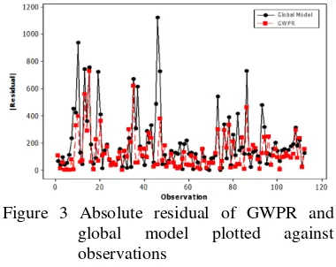
The performance of GWPR model compared to the global model also can be seen from the residual values. According to Figure 3, residual of GWPR model is relatively less than global model for each region. The total absolute residual value is 14,467.94 for GWPR model and 22,020.07 for the global model. Similar with the AICc difference, the difference of the total absolute residual value for two models was very high. Therefore GWPR model will be considered as the best model.

Figure 3 Absolute residual of GWPR and global model plotted against observations

Stationary Parameter and Fitted Model of GWPR

The method used to test the stationarity in GWPR parameters is done by comparing the inter-quartile range of GWPR model and the standard error of the global model. If the local inter-quartile range (IQR) is twice the global standard error or more, then the variable requires a non-stationary model to represent it adequately (Cheng et al. 2011).

from four aspects and how it varies over space in relation to deprivation conditions regionally.

Table 5 Simple test for non-stationary parameter estimate

Variable Standard Error (Global model)

IQR (GWPR) Intercept 0.010759 0.237853 FamLabour 0.000000* 0.000003

FamRiver 0.000002 0.000031

FamSlums 0.000001 0.000094

ISP 0.000008 0.000377

Doctor 0.000019 0.001992

DiffPlace 0.000266 0.010788

JHSch 0.000059 0.002455

* value in 10 digit decimals is 0.0000000089 The final fitted model of GWPR is given as:

ln ̂ i = ̂0(ui,vi) + ̂1(ui,vi) FamLabour + ̂2(ui,vi) FamRiver – ̂3(ui,vi) FamSlums + ̂4(ui,vi) ISP – ̂5(ui,vi) Doctor

+ ̂6(ui,vi) DiffPlace – ̂7(ui,vi) JHSch (5) The symbol of (ui,vi) besides the parameter estimates in equation (5) defined that the

parameter estimates is in a non-stationary condition. Summary of statistics for varying (local) coefficients are shown in Appendix 6.

Spatial Variability Map

Concerning the individual significance of the parameters, though they are all statistically significant in the global regression, there are several non-significant parameters in the GWPR models. Therefore, spatial variability map is needed. GWPR parameter estimates map has some advantages. First, the map provides specific information for each area including parameter estimates which are calculated in the case of global models. Second, the map also can lead to some regions which have highly relation to dependent variable for each explanatory variable.

10

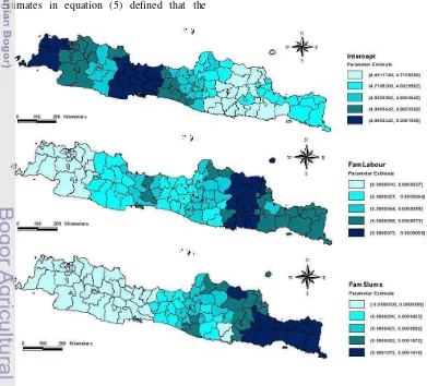
Figure 4 Map of eight parameter estimates of GWPR model The local parameter estimates of intercept

were very high in the regencies and cities in border area of West Java and Central Java province, and also in all of regencies and cities in Banten province. This indicate that the higher malnourished patients in this regions when the other variables are constant. However, they were pretty low in most of the

regencies and cities in border area of Central Java and East Java province and it indicates the low relation to the malnourished patients.

of West Java province. The map shows that all of the local parameter estimates of FamLabour variable are positive. This indicated that increasing the number of families whose members are farm labour would increase the number of malnourished patients for each region. One of the recommendation to the local or central government is to make a welfare programme for farm labours which indirectly decrease the poor people. This programme might decrease the number of malnourished patients for each region.

Next, the local parameter estimates of FamRiver were pretty low in Banyumas, Banjarnegara, Pekalongan, Tegal, Purbalingga regency, Tegal, Pekalongan city, and all of the regencies and cities in the central and east area of East Java province. However, the parameter estimates in the regions of Rembang, Blora, Tuban, Bojonegoro, and most of the regencies and cities in West Java province were very high. The higher value of local parameter estimates indicated that these regions would have a higher increase of malnourished patients. Therefore, the regions with high parameter estimates must be given a solution for this problem by the government, especially local government. For example, the local government in these regions might build more flat house units like in DKI Jakarta to relocate the families residing along the river. This recommendation is expected to decrease the number of malnourished patients.

In FamSlums variable, the parameter estimates of all of the regencies and cities in the central and western area of East Java and Tuban regency were very high. However, the regencies and cities in West Java, DKI Jakarta, Banten province, some regencies and cities in the west region of Central Java province, Ponorogo, and Trenggalek regency have a pretty low negative local parameter estimates. Their negative value indicated that increasing the number of families residing in the slums would decrease the number of malnourished patients. It was clear that poverty aspect in general can increase the number of malnourished patients. Therefore, the FamSlums as one of the representation of poverty aspect had a different expectation because of the negative value of its local parameter estimates. It might be caused that in these regions were not often recorded malnourished patients.

The FamRiver variable was the highest influencing factors to the number of malnourished patients compared to the other variables which represent the poverty aspect,

which is based on the comparisson of the mean of local parameter estimates from FamLabour, FamRiver, and FamSlums variable according to Appendix 6. This indicated that the regions with high number of families residing along the river must be given the serious attention by local government.

All of the local parameter estimates in ISP variable were positive. This indicated that the number of integrated services post (Posyandu) in each region are positively related to the expected number of malnourished patients. The possible reason is that increasing of integrated services post (Posyandu) units, which have been built by the government, through the Ministry of Health in each region was done without considering that a region is an endemic area or not to malnutrition case. The other reason is that increasing the number the integrated services post (Posyandu) in a region may cause the detection of many malnourished patients. These patients are also allowed to have a consultation about malnutrition to the health workers in Posyandu.

Then, the local parameter estimates of Doctor were low and negative in Ciamis regency, Banjar city, and all of the regencies and cities in Central Java, East Java, and DI Yogyakarta province. In these regions, increasing the number of doctors would decrease the expected number of malnourished patients. This condition may be used as a recommendation to the government that these regions need additional health workers, especially doctors in order to decrease the malnutrition case. However, the local parameter estimates of Doctor variable were positive in the other regions. If we look into the map of parameter estimate in Doctor variable, the regions with positive local parameter estimates includes all of regencies or cities in DKI Jakarta, Banten, and most of the regions in West Java province. In these regions it was possible that the need of the number of doctors was high, especially in big cities like in DKI Jakarta province.

12

representation did not have a direct influence to the number of malnourished patients.

The last variable is DiffPlace. All of the regencies and cities in Central Java and DI Yogyakarta have positive local parameter estimates. The model indicated that increasing the total village having insufficient access towards the village office and the capital of sub-district would increase the expected number of malnourished patients. Meanwhile, for other regions, DiffPlace variable was negatively related to the number of malnourished patients. It might be caused by more sufficient access towards the village office and the capital of sub-district, so there are many malnourished patients being recorded by the local government official workers, especially by the health workers.

The local parameter estimates that were inversely related with some variables might produce bad interpretation. For better results of GWPR model, the study of regions for the next research should be done at a lower, such as be sub-district or village level. Using lower levels might enhance the precision of parameter estimates in spatial analysis.

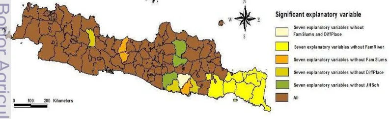
Significant Explanatory Variables Map GWPR model usually displays the map of non-stationary parameter estimates. However, in every point of the regression, in this case each regency or city, it also has a pseudo t -value which is formulated as by the parameter estimate divided with the standard error in each point of the regression. As a result, the GWPR local parameters of explanatory variables (we exclude the intercept) have t-maps (Mennis 2006). Each t-map has an advantage that is it can detect the significancy of an explanatory variables for each region. The other advantage is it can detect the

combination of significant explanatory variables for each region. But, the disadvantage of this mapping approach is that potentially interesting patterns may not be observed regarding the magnitude of the relationship between the explanatory and dependent variable as contained in the actual parameter estimate values, as well as in the magnitude of the significance (Mennis 2006).

In this research, every t-map of GWPR local parameter of explanatory variable would be joined as a map which is named as map of significant explanatory variable. Figure 5 shows the significant explanatory variable map. The explanatory variables used in the map are the explanatory variables used in the selected global model.

The map in Figure 5 displays six groups of color. The colors indicate that there were different groups without implaying a rank like the map in Figure 4. The dominant color was dark brown, it indicates that in these regions, all of the explanatory variables were significant. A region where FamSlums and DiffPlace variable were not significant is Ponorogo regency. Tulungagung, Pacitan, and Majalengka regency only had DiffPlace variable as a significant variable. Then, FamRiver variable was significant in eastern area of East Java. FamSlums variable was not significant in Pemalang, Trenggalek, and Purbalingga regency. The last group is the regions which JHSch was not a significant variable. The regions include Blora, Wonogiri, and Ngawi regency. The other advantage for creating this map is it can give recommendations for policy maker or the local government and central government especially Ministry of Health about the factors influencing the number of malnourished patients in each regency or city in Java island.

CONCLUSION AND RECOMMENDATION

Conclusion

GWPR model was proven to be a better model than global model. GWPR model had highly difference of AICc compared to the global model. A condition of non-stationarity in parameters was fulfilled, and its residual relatively less than global model for each region. Map of parameter estimates showed more meaningful results. The FamRiver variable was the highest influencing factors to the number of malnourished patients compared to the other variables which represent the poverty aspect. There were six groups of the factors influencing the number of malnourished patients for each regency and city in Java based on the map of significant explanatory variable.

Recommendation

For better results of GWPR model, the study of regions for the next research should be lower level than regency or city level, such as the sub-district or village level. Conducting GWPR at this level might give a better local parameter estimates.

REFERENCES

A’yunin Q. 2011. Modeling of Malnutrition Infants Under Five (Toddlers) in Surabaya with Spatial Autoregressive Model (SAR) [Minithesis]. Surabaya: Undergraduate Programme, Institut Teknologi Sepuluh November.

Anselin L. 1999. Spatial Econometrics. Bruton Center: University of Texas. TX 75083-0688.

Arbia G. 2006. Spatial econometrics:

Statistical Foundations and Applications

to Regional Convergence. Berlin: Springer

Publishing.

Aulele SN. 2010. Geographically Weighted Poisson Regression Model (Case Study: The Number of Infant Mortality in East Java and Central Java 2007) [Thesis]. Surabaya: Postgraduate Programme, Institut Teknologi Sepuluh November. Burnham and Anderson (1998). Model

selection and multimodel inference: a practical information-theoretic approach. New York: Springer Publishing.

Cameron AC and Trivedi PK. 1998. Regression Analysis of Count Data. Cambridge: Cambridge University Press.

Charlton M and Fotheringham AS. 2009. Geographically Weighted Regression White Paper [Paper]. Maynooth: Science Foundation Ireland.

Cheng EMY, Atkinson PM, and Shahani AK. 2011. Elucidating the spatially varying relation between cervical cancer and socio-economic conditions in England, International Journal of Health Geographics, 10:51.

C:\data\StatPrimer\correlation.wpd. http:// www.sjsu.edu/faculty/gerstman/StatPrimer /correlation.pdf. [September 12th, 2012] Directorate of Public Health Nutrition. 2008.

Pedoman Respon Cepat Penanggulangan Gizi Buruk. Jakarta: Ministry of Health Republic of Indonesia.

Fleiss JL, Levin B, and Paik MC. 2003. Statistical Methods for Rates and Proportions 3rd Ed. New York: Columbia University.

Fotheringham AS, Brunsdon C, and Charlton M. 2002. Geographically Weighted Regression: The Analysis of Spatially Varying Relationship. Chichester: John Wiley and Sons, ltd.

Hardin JW and Hilbe JM. 2007. Generalized Linear Models and Extensions. Texas: A Stata Press Publication.

Http://www.ppjk.depkes.go.id/index.php?opti on=com_content&task=view&id=53&Item id=89. [November 25th, 2012]

Long JS. 1997. Regression Models for Categoricals and Limited Dependent Variables. California: SAGE Publications. Mennis J. 2006. Mapping the Results of

Geographically Weighted Regression, The Cartographic Journal, 43(2):171–179.

Nakaya T, Fotheringham AS, Brunsdon C, and Charlton M. 2005. Geographically Weighted Poisson Regression for Disease Association Mapping, Statistics in Medicine, 24:2695-2717.

National Institute of Health Research and Development. 2008. Laporan Hasil Riset Kesehatan Dasar (Riskesdas) Nasional. Jakarta: Ministry of Health Republic of Indonesia.

Rohimah SR. 2011. Spatial Autoregressive Poisson model for Detecting the Influential Factors of the number of Malnourished patients in East Java [Thesis]. Bogor: Postgraduate Programme, Bogor Agricultural University.

14

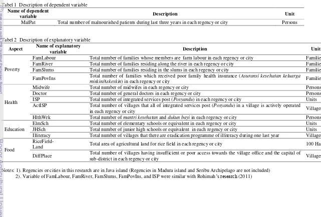
Appendix 1 Description of dependent variable and explanatory variables Tabel 1 Description of dependent variable

Name of dependent

variable Description Unit

MalPat Total number of malnourished patients during last three years in each regency or city Persons

Tabel 2 Description of explanatory variable Aspect Name of explanatory

variable Description Unit

Poverty

FamLabour Total number of families whose members are farm labour in each regency or city Families

FamRiver Total number of families residing along the river in each regency or city Families

FamSlums Total number of families residing in the slums in each regency or city Families

FamPovIns Total number of families which received poor family health insurance (Asuransi kesehatan keluarga _{miskin/Askeskin}

) in each regency or city Families

Health

Midwife Total number of midwifes in each regency or city Persons

Doctor Total number of general doctors in each regency or city Persons

ISP Total number of integrated services post (Posyandu) in each regency or city Units

ActISP Total number of villages that all of integrated services post (Posyandu) in a village is actively operated

in each regency or city Villages

HlthWrk Total number of mantri kesehatan and dukun bayi in each regency or city Persons

Education

ElmSch Total number of elementary schools or equivalent in each regency or city Units

JHSch Total number of junior high schools or equivalent in each regency or city Units

Illiteracy Total number of villages that there are eradication programme of illiteracy during one last year Villages

Food

RiceField-

Land Total area of agricultural land for rice field in each regency or city 100 Ha

DiffPlace Total number of villages having insufficient or poor access towards the village office and the capital of

sub-district in each regency or city Villages

Notes: 1). Regencies or cities in this research are in Java island (Regencies in Madura island and Seribu Archipelago are not included)

16

Appendix 2 Algorithm of research method

1

Appendix 3 Map of malnourished patiens distribution for each regency and city in Java island (2008)

Note: unit of malnourished patiens in persons

18

Appendix 4 Boxplot of dependent variable and explanatory variables

Notes:

1. Poverty aspect: FamLabour, FamSlums, FamRiver, and FamPovIns variable 2. Health aspect: ISP, ActISP, Doctor, Midwife, and HlthWrk variable 3. Education aspect: ElmSch, JHSch, and Illiteracy variable

4. Food aspect: RiceFieldLand and DiffPlace variable

1

Appendix 5 Pearson’s correlation between variables (dependent variable and explanatory variables)

MalPat FamLabour FamRiver FamSlums FamPovIns Illiteracy ISP ActISP RiceField-

Land Doctor Midwife HlthWrk DiffPlace ElmSch FamLabour 0.586

FamRiver 0.455 0.402

FamSlums -0.102 -0.104 0.323

FamPovIns 0.759 0.615 0.336 -0.188

Illiteracy 0.674 0.676 0.423 -0.124 0.628

ISP 0.841 0.690 0.422 -0.105 0.891* 0.741*

ActISP 0.788 0.728* 0.377 -0.177 0.837* 0.783* 0.897*

RiceField-

Land 0.749 0.585 0.335 -0.214 0.795* 0.706* 0.787* 0.877*

Doctor 0.567 0.362 0.275 0.097 0.478 0.358 0.640 0.394 0.265

Midwife 0.815 0.697 0.396 -0.102 0.843* 0.759* 0.960* 0.914* 0.799* 0.635

HlthWrk 0.798 0.737* 0.442 -0.161 0.881* 0.791* 0.938* 0.927* 0.844* 0.464 0.913*

DiffPlace 0.340 0.377 0.257 -0.049 0.296 0.396 0.316 0.350 0.288 0.204 0.390 0.369

ElmSch 0.608 0.826* 0.594 0.195 0.666 0.676 0.735* 0.768* 0.633 0.345 0.730* 0.780* 0.327

JHSch 0.426 0.632 0.635 0.368 0.461 0.505 0.552 0.558 0.430 0.241 0.543 0.625 0.304 0.900*

*|r|≥0.7 is strong Correlation (source: C:\data\StatPrimer\correlation.wpd). Underlined variable is dependent variable.

20

Appendix 6 Summary statistics for varying (local) coefficients

Variable Mean Std. Dev. Min. Q1 Q2 Q3

Intercept 4.817929 0.164236 4.601174 4.716957 4.871907 4.954810 FamLabour 0.000005 0.000002 0.000001 0.000003 0.000005 0.000006 FamRiver 0.000052 0.000024 -0.000010 0.000038 0.000053 0.000069 FamSlums 0.000033 0.000055 -3.20x10-5 -0.000025 0.000036 0.000069 ISP 0.000858 0.000212 0.000406 0.000674 0.000940 0.001051 Doctor -0.000710 0.000924 -0.001850 -0.001490 -0.001271 0.000502 DiffPlace -0.001510 0.005036 -0.010250 -0.006885 -0.003167 0.003903 JHSch -0.002040 0.001421 -0.005300 -0.002985 -0.002292 -0.000529

Variable Max. Range IQR