KINEMATIC SYNTHESIS OF PLANAR, SHAPE-CHANGING RIGID BODY
MECHANISMS FOR DESIGN PROFILES WITH SIGNIFICANT DIFFERENCES IN ARC
LENGTH
Shamsul A. Shamsudin∗ Andrew P. Murray
David H. Myszka
Design of Innovative Machines Laboratory (DIMLAB) Department of Mechanical and Aerospace Engineering
University of Dayton Dayton, Ohio 45469
Email: [email protected] [email protected]
James P. Schmiedeler
Department of Aerospace and Mechanical Engineering University of Notre Dame
Notre Dame, Indiana, 46556 Email: [email protected]
ABSTRACT
This paper presents a kinematic procedure to synthesize pla-nar mechanisms capable of approximating a shape change de-fined by a general set of curves. These “morphing curves”, re-ferred to as design profiles, differ from each other by a com-bination of displacement in the plane, shape variation, and no-table differences in arc length. Where previous rigid-body shape-change work focused on mechanisms composed of rigid links and revolute joints to approximate curves of roughly equal arc length, this work introduces prismatic joints into the mechanisms in or-der to produce the different desired arc lengths. A method is presented to inspect and compare the profiles so that the regions are best suited for prismatic joints can be identified. The result of this methodology is the creation of a chain of rigid bodies con-nected by revolute and prismatic joints that can approximate a set of design profiles.
INTRODUCTION
Certain mechanical systems benefit from the capacity to vary between specific shapes in a controlled manner. Consider the
ad-∗Address all correspondence to this author.
vantages of an aircraft wing that can change between different profiles for loiter versus attack modes. Weishaar [1] highlights the military’s search for technology that will enable wings to ac-tively change shapes in order to achieve wider ranges of aerody-namic performance and flight control than are possible with the current conventional wing technology. Other mechanical sys-tems that can benefit from being able to adapt (or morph) and maintain prescribed shapes include smart aperture antennas [2] and deployable membrane mirrors [3].
Different methods can be used to achieve a morphing ca-pacity, such as compliant mechanisms and shape memory alloy materials. Kota and his colleagues [4, 5] used optimization algo-rithms to search discrete characteristics of a topology to best uti-lize compliant mechanisms. They studied how compliant mech-anisms could control the change of shape of a parabolic antenna. Concerns with these methods include cost and the magnitude of achievable displacements. Shape-changing rigid-body mecha-nisms have been proposed as an alternative to the above tech-nologies with the advantage of lower cost, greater displacements and higher load carrying capabilities. Additionally, rigid-body linkages have a well established set of mechanical design prin-ciples. Rigid-body shape change has been applied to open curve Proceedings of the ASME 2011 International Design Engineering Technical Conferences &
Computers and Information in Engineering Conference IDETC/CIE 2011 August 28-31, 2011, Washington, DC, USA
A shape-changing design problem is posed by specifying a set of design profiles, such as wing profiles for loiter and attack modes. The synthesis process begins by representing each of the design profiles in a standardized manner, such that comparisons can be made among the set. The standardized representations of the design profiles are called target profiles. The process contin-ues with a segmentation phase that creates segments, which are generated in shape and length so that they form rigid links that approximate corresponding portions on each target profile. To complete the synthesis, a mechanization phase adds binary links to each segment in order to achieve a lower degree-of-freedom (dof) linkage. If possible, a system with a single dof is pre-ferred for simplicity in control. The currently available synthesis method addresses problems with profiles of roughly the same arc length [6, 7]. This is a serious limitation for general design prob-lems.
This paper presents enhancements to the rigid-body shape-change theory that enable the matching of design profiles with significant differences in arc length. These developments alter the segmentation methodology to introduce prismatic joints into the chain of bodies used to approximate a set of design profiles. The remainder of the paper is organized as follows. Section 2 addresses a new process for converting design profiles into target profiles having similar spacing between definition points. Simi-lar spacing is necessary in order to compare regions of the pro-files with different lengths. Section 3 presents a strategy for de-termining the curvature of, smoothing and regenerating the tar-get profiles. Understanding the curvature of the profiles assists in identification of regions ideally suited for a prismatic joint. Section 4 discusses the process for comparing target profile cur-vatures to allow for the introduction of prismatic joints. Section 5 describes how the remaining segments of the design curves are approximated with rigid bodies connected by revolute joints and gives a mechanization example to generate a single-dof linkage.
1 Creating Target Profiles
The shape-change problem is posed by specifying a set ofp design profiles that represent the different shapes to be attained by the mechanism. Murray et al. [6] define a design profile jas an ordered set ofNjpoints for which the arc length between any
two can be determined. Typically, each design profile is viewed as piecewise linear [8]. Theith point on the jth design profile is designatedaji,bji
T
. The length of theith piece on the jth design profile is
cji= q
aji+1−aji 2
+ bji+1−bji 2
, (1)
Cj=
Nj−1
∑
i=1
cji. (2)
The design profiles may be defined by any number of points spaced at various intervals, producing a wide range of cji. To
proceed with kinematic synthesis, the design profiles are con-verted to target profiles that have common features. It is impor-tant for the target profiles to have common features so compar-isons can be made and a chain of rigid-bodies can be formed that when repositioned will approximate all design profiles. In earlier work [6, 7], the design profiles were assumed to be of roughly equal arc lengths,C1≈C2≈. . .≈Cp. In that case, the design
profiles could be converted to target profiles that all have the samennumber of defining points distributed equally along the design profile so that each segment has roughly the same length, cji≈ckl,∀i,j,k,l.
Constant piece lengths dictate equally spaced points and al-low for identification of corresponding points on each target pro-file. Shape approximation relies on comparing groups of corre-sponding points. For the work in this paper, the profiles may possess large differences in arc length. In order to maintain a constant piece length, the design profiles are now converted to target profiles that each may have a different number of points nj. By specifying a desired piece lengthsd, the number of
seg-mentsmj on profile j can be determined. Smaller values ofsd
produce more linear pieces and smaller variations between the design and target profiles.
The number of linear pieces must be an integer and an initial value is calculated as
mj=
Cj sd
, (3)
where⌈ζ⌉represents the ceiling function, which is the smallest integer not less thanζ. Thus, the ratio of Eq. 3 will be rounded upward, producing a greater number of target profile pieces that are shorter than, or equal to,sd. The corresponding number of
points on the target profile jis
nj=mj+1. (4)
Provisional target profiles are generated by distributing nj
points at increments ofCj/mj along the jth design profile. The jthtarget profile becomes a piecewise linear curve composed of line segments, called pieces, connecting the ordered set of points zji =
xji,yji T
FIGURE 1: Design profile (solid) with an approximating target
profile (dashed) where points are positioned to give a constant arc length along the design profile.
on the jthtarget profile is
sji =
The distribution of target profile points along a design profile is shown in Fig. 1. Since the points on the jth target profile are separated by equal arc lengths ofCj/mjalong the design profile, sji will not necessarily be constant. With Eq. 3 specifyingmj≥
Cj/sd,sji≤sd∀i=1, ...,mj,j=1, ...,nj.
The average linear piece length for the jthprofile is
¯
An error representing the difference between the average seg-ment length and desired segseg-ment length is calculated as
Esj= sd−s¯j
. (7)
An iterative procedure decreasesnjby 1 and redistributes points
along the design profile to create a new target profile. Points are removed until then∗j (and correspondingly, m∗j) that minimizes Esj is reached. The end result is that a minimal number of points
n∗j are used to construct the jth target profile such that all
lin-ear piece lengths are approximately equal to the desired segment length.
Applying this process to all design profiles,ptarget profiles are constructed such that all linear pieces have lengths that are approximately equal tosd. The average length of all linear pieces
on all profiles is
¯
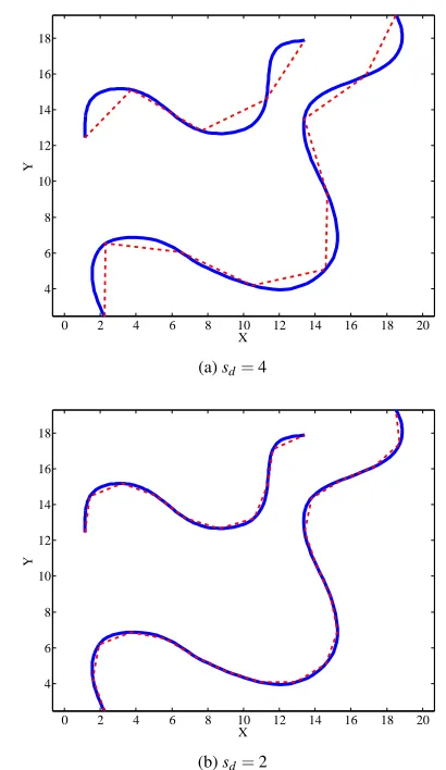
FIGURE 2: Target profiles (dashed) havingsd=4 poorly
ap-proximate design profiles (solid), whereas target profiles having sd=2 create a much better approximation.
Note that ¯smis governed by the choice ofsdthrough Eqs. 7
and 8. As in the previous work, the heuristic employed is to select sd such that the target profile arc length is greater than
99% of the design profile arc length,m∗jsd>0.99Cj, j=1. . .p.
Figure 2 illustrates two target profiles. In Fig. 2a,sd=4 results
in target profiles that poorly approximate the design profiles. In Fig. 2b, sd=2 results in target profiles that exhibit significant
improvement in approximating the design profiles.
2 Curvature Calculations
2.1 Calculating the Curvature of Target Profiles
Excluding the first and last points, the curvatureκjiof thej th
target profile at theith point can be determined by constructing
an arc that passes through zji and the neighboring pointszji−1
andzji+1 [9]. The curvature has a magnitude that is the inverse
of the radius passing through the three points,
κji=
, and the general equation of that circle
(x−αji)
2+ (y−β ji)
2=r2
ji can be expanded and rewritten
(r2ji−α2ji−β 2
ji) +2xαji+2yβji =x 2+y2.
(10)
Substituting the coordinates of the three points into Eq. 10, the three equations can be expressed in matrix form [10]
rji. Further substitution into Eq. 9 determines the curvatureκji
of the target profile atzji.
The sign of curvatureκji is designated positive ifzji−1,zji
andzji+1 form a counterclockwise turn and is determined from
direction vectors [11,12]. A direction vectorPji−1is defined such
that it extends fromzji−1 tozji.
is positive, the curvature is
desig-nated positive, and vice versa [13].
The first and last points of any profile have no curvature. In order to apply the curvature smoothing algorithm that is de-scribed in the next section, the first point is taken to have the curvature of the second point and the last point that of the second to last point. Thus,κj1 =κj2andκjn∗j =κjn∗j−1.
the target profiles. Since large-scale matching of the profiles is desired, smoothing of the curvatures is accomplished with a weighted moving average technique [14, 15]. Excluding the first and last points, the smoothed curvature of the jthtarget profile at theithpoint is calculated as
˜
The smoothed curvatures of the first and last points are calculated as
Successive passes through the smoothing function will con-tinue to decrease the scatter of the curvature. Unlike increasing the half-width of the moving average, this method preserves cur-vature data at the end of the profiles. Additionally, repeatedly applying the smoothing function allows the designer to assess the acceptability of the curvature information after each pass.
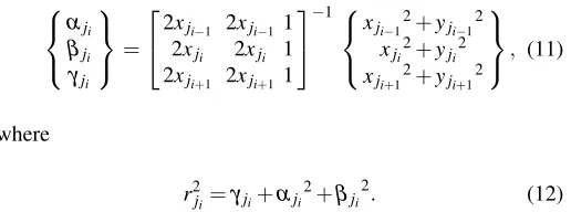
Two target profiles are shown as the solid curves in Fig. 3a. The curvature calculated from Eqs. 9, 11, and 12 is shown in Fig. 3b. The smoothed curvature calculated with five iterations through Eqs. 14, 15 and 16 is shown in Fig. 3c. It is noted that the smoothed curvature plot has less scatter and provides a better instrument to identify regions of similar curvature.
2.3 Regenerating the Target Profile
The target profiles are regenerated using a constant piece length of ¯sm and the smoothed curvature data. This ensures a
constant spacing between points along the target profile and vi-sually confirms that smoothing does not dramatically influence the accuracy of the shape change curves. Specifically, the loca-tion of a regenerated point ˜zji+1 is constructed from ˜zji−1, ˜zji and
and is determined by using the equation of a circle,
0 5 10 15 20
FIGURE 3: Target profiles (a) with calculated curvature (b) and
smoothed curvature (c). The dashed curves in (a) are regenerated profiles and are nearly identical to the original profiles.
pressing in matrix form generates two equations,
satisfy Eqs. 18. The sign of ˜rji is used to identify the correct center point.
Since ˜zji+1 also shares the center point, substituting into
Eq. 17 gives
The regenerated target profiles are constructed with constant lin-ear piece length ¯sm. Thus, ˜zji+1 will be spaced a distance ¯smfrom
Equations 19 and 20 can be reduced into a second order equation that will produce two sets ofx˜ji+1,y˜ji+1
T
. One solution will be identical to
˜ xji−1,y˜ji−1
T
, which is discounted, leaving one acceptable solution. Figure 4 illustrates the graphical solution to Eqs. 19 and 20. Thus, the location of ˜zji+1 is regenerated from
˜
zji−1, ˜zji and ˜κji.
Starting with points 1 and 2, where ˜zj1=zj1 and ˜zj2 =zj2,
as the solid curves in Fig. 3a, whereas the dashed curves repre-sent the regenerated profiles using the smoothed curvature, con-firming only minor deviation.
3 Selection of Prismatic Joints
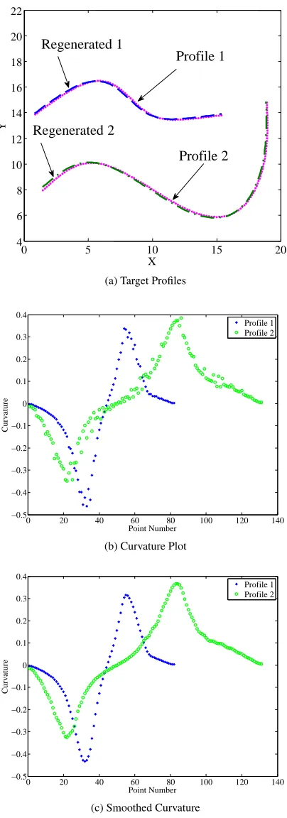
The segmentation process identifies subsets, or segments, of each target profile to form rigid links. The process of creat-ing segments starts with two points on a reference target profile. Corresponding segments on the other profiles are then created that have the same number of points as the reference segment. Murray et al. [6] developed a method, as illustrated in Fig. 5, to translate and rotate segments such that the sum of the distances between each point on the target segment and the corresponding point on the reference segment is minimized. A mean segment is constructed by determining the geometric center of the set of pcorresponding points on the shifted segments. The mean seg-ment curve is shifted back to the original location of profiles 2 through p and represents one rigid-link in the shape-changing chain. The process is repeated by adding one point at a time to the segment until the maximum error between a mean segment point and a target profile point remains below the allowable er-ror. At that stage, the mean segment becomes the first rigid-body. This iterative process is repeated to create the next rigid-body. A small point-to-point error typically produces more, smaller seg-ments. However, the better approximation is offset with mechan-ical complexity.
When the design curves have significantly different arc lengths, each target profile is defined with a different number of points. This situation is illustrated in the curvature plots of Fig. 3c, where profile 1 contains 82 points, while profile 2 con-tains 132. Prismatic joints included along the rigid-body chain can absorb the additional 50 points, thereby accommodating the different profile lengths. Mechanically, this is accomplished by connecting two rigid bodies of the same curvature with a pris-matic joint that allows the length across the two bodies to vary.
In this work, the prismatic joints are constrained to follow a constant radius trajectory. Regions on the target profiles that have approximately constant and equal curvature are ideal for inserting two rigid links connected with a prismatic joint. The constant and equal curvature criteria are assessed by observing a plot as shown in Fig. 3c. A curvature band, as shown in Fig. 6, is selected by the designer to identify regions along each profile that have nearly constant curvature. In Fig. 6, 7 points from profile 1 and 35 points from profile 2 are included within the selected curvature band. This is a prime location for two links that will be joined with a prismatic joint. Recall that profile 2 is longer and therefore should have more points that are included in the curvature band.
When specifying regions of the target profiles that will be
0 2 4 6 8
0 1 2 3 4 5 6 7 8
0 2 4
0 1 2 3 4 5 6 7 8
0 2 4
0 1 2 3 4 5 6
0 2 4 6 8
0 1 2 3 4 5 6
Reference Profile Profiles
Mean Profile
(a) (b)
(c) (d)
FIGURE 5: (a) Three segment curves are represented by one
mean segment. (b) Two segments are transformed together to the third according to minimized distance among points. (c) The av-erage position among corresponding points forms the mean seg-ment. (d) The mean segment is transformed back to the original segment positions. Adapted from [6].
approximated with a pair of rigid links joined with a prismatic joint, a common starting point must be selected. This ensures that the portion of the target profiles leading up to the selected point have the same arc length and can be approximated with a chain of rigid links joined with revolute joints. Separate ending points are selected to designate the region on each profile that will be approximated with a pair of links joined with a prismatic joint. The ultimate goal is to assign more points to the prismatic joint stroke on the longer profile(s).
Multiple prismatic joints may be necessary to compensate for the differences in target profile lengths. The starting point on theethcurvature band of the jth profile is designated askej and
0 20 40 60 80 100 120 140 −0.5
−0.4 −0.3 −0.2 −0.1 0 0.1 0.2 0.3 0.4
Point Number
Curvature
Good curvature band
Common start point selected End point for bodies with prismatic joints on profile 1
End point for bodies with prismatic joints on profile 2
FIGURE 6: Design profile (solid) with approximating target
pro-file (dashed) where points are positioned to give a constant seg-ment length.
radius of theethband on all target profiles is
rme= p
∑
j=1 nej
p
∑
j=1 ke j+me j
∑
i=ke j
˜ κji
. (21)
This mean radius defines the best-fit, single arc of a curved prismatic joint. The arc length across the two links that will be connected by theethprismatic joint on thejthprofile is calculated as
Lej=mejsm, (22)
where
mej =nej−1. (23)
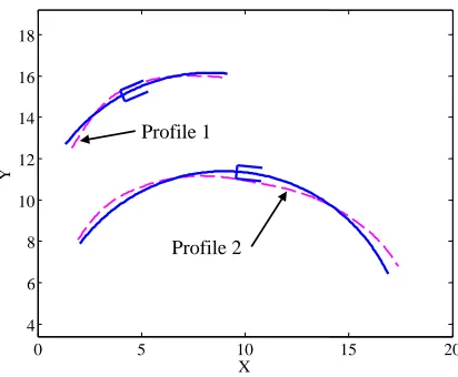
The arc is placed in the selected region on each target profile such that the least-squares distance from the arc to each point on the target profile is minimized. Figure 7 illustrates two tar-get profiles of different lengths. Arcs, both with radiusrm1, and
lengths of L11 andL12 are fit through the profiles. Links
con-nected by a prismatic joint constrained to move along this arc
0 5 10 15 20
4 6 8 10 12 14 16 18
X
Y
Profile 2 Profile 1
FIGURE 7: A prismatic joint is placed onto two target profile
segments with nearly equal and constant curvature.
produce a rigid-body chain that is capable of changing between the two profiles.
After a set of curvature bands is selected, the arc length of the remaining portions of the profiles must be determined. As stated, if arc length differences still exist, an additional prismatic joint is required. Across all target profiles, the start of the next curvature band must be the same number of points from the end of the previous curvature band. This ensures that rigid bodies, joined with revolute joints, can approximate the portions of pro-files between curvature bands.
With each additional prismatic joint, a new curvature plot that begins at the final point of the previously selected curva-ture band is created for each target profile. Figure 8 shows a re-aligned curvature plot derived from Fig. 6 after selecting the first set of curvature bands. Since profile 2 is still visibly longer than profile 1 (59 points compared to 32 points), a second curvature band must be selected for including prismatic joint. The selec-tion method is repeated to locate regions on each profile where the next prismatic joint should be placed.
Curvature bands are selected untilqprismatic joints are in-cluded in the shape-changing chain such that on each profile, the number of points not included in curvature bands are equal. That is,
m1−
q
∑
e=1
me1 =. . .=mj− q
∑
e=1
mej =. . .=mp− q
∑
e=1 mep.
(24)
4 Forming the Remaining Rigid Links
con-FIGURE 8: In order to identify a potential region in which to insert another prismatic joint, the curvature distribution (from Fig. 6) is replotted starting with the end of the previously se-lected curvature band.
trolled by a user-determined error value, which is the maximum point-to-point distance from the mean segment to each shifted target profile (see Fig. 5c). The objective is to divide the target profile into segments that reduce the error in approximating the design profiles.
As instances of the mean segment are shifted back to the original location of each profile, the end points of each segment in the chain do not coincide. To join the segments with a revolute joint, the end points must be adjusted to become coincident. The previous synthesis process used an optimization procedure to re-locate the start and end points for each segment such that each adjustment across all profiles is minimized.
In creating the segments for profiles of various lengths, the links to be joined with a prismatic joint are identified through the selection of appropriate curvature bands. The ranges of prismatic sliding are placed on the target profiles as shown in Fig. 9. The remaining portions of the target profiles will have approximately the same number of points and hence the same length, as dictated by Eq. 24. These portions of the target profiles can be matched with rigid links connected by revolute joints.
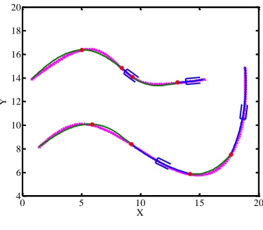
Close inspection of Fig. 9 shows that the end points of the mean segments are not coincident. As stated, previous work used an optimization procedure to relocate the start and end points for each segment and form a revolute joint. The work presented in this paper uses an alternate process to avoid the time con-straints imposed by the numerical complexities of optimization. A straight “pointing line” is constructed by connecting the start and end points of the first segment on each profile, as shown in Fig. 10. The first point of each instance of the first mean segment is placed at the start of each target profile. Then, each instance of the mean segment is rotated until its endpoint lies on the
point-0 5 10 15 20
4 6 8 10 12 14 16 18 20
X
Y
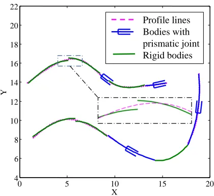
Bodies with prismatic joint Rigid bodies
FIGURE 9: The mean profile is segmented into rigid bodies
based on a user-defined error and placed to minimize the point distance from the target profile. The allowable point-to-point error in this case is 0.15 unit.
ing line. This endpoint locates the first revolute joint that will connect to the second mean profile.
In locating the second rigid body, a second pointing line is constructed from the first revolute joint to the endpoint of the second segment on each target profile. The first point of each instance of the second mean segment is placed at the first revo-lute joint of each target profile. As before, each instance of the second mean segment is rotated so that its ending point lies on the pointing line. Again, the endpoint locates the revolute joint that will connect to the third mean profile. Figure 10 illustrates this concept of constructing pointing lines and locating revolute joints.
Once the revolute joints are located, a chain of rigid links joined with revolute and prismatic joints are placed on the target profile. This chain can be repositioned to approximate all tar-get profiles. Figure 11 shows two instances of the same chain that approximates the different length profiles. The blue mem-ber represents two rigid bodies joined with a prismatic joint, which is constrained to a constant radius trajectory. Notice that a smaller specified error creates a greater number of segments and improves the accuracy of the shape-change approximation as shown in Figs. 11a and 11b.
FIGURE 10: Pointing lines are used to move the ends of the seg-ments moved to a common point and form a revolute joint.
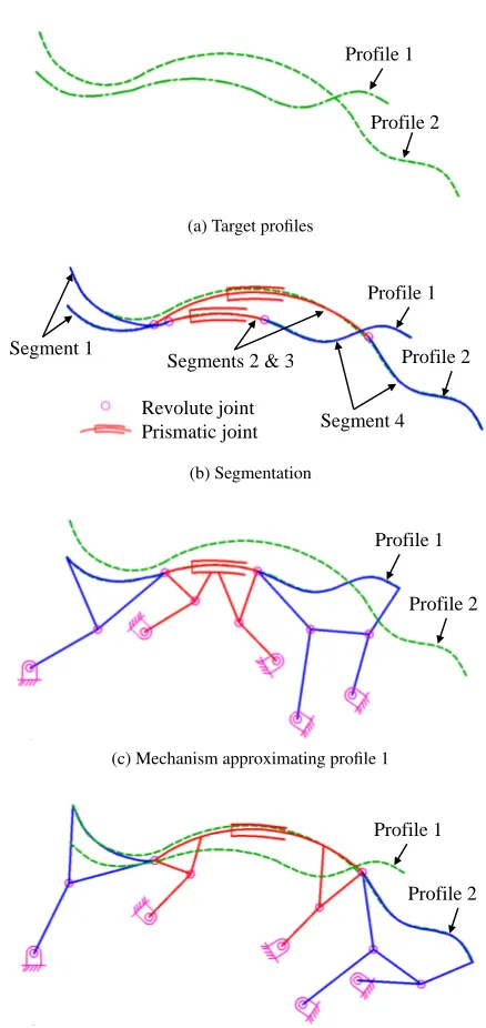
that is able to alter its shape between the two profiles in Figs. 12c and 12d.
5 Conclusion
This paper presents theory and a strategy to synthesize pla-nar rigid-bodies that are capable of approximating shape changes defined by a general set of different length curves. Design curves are specified based upon the necessary task. Earlier work rep-resented design curves with target profiles that have the same number of equally spaced points on each profile because equally spaced points are important to make comparisons among the pro-files. With design curves that have different lengths, this paper presents a strategy to generate target profiles that have a different number of equally spaced points on each profile, controlled by a desired linear piece lengthsd.
The main contribution of this paper is the inclusion of pris-matic joints within the chain of rigid bodies that accomplishes shape change tasks. Curvature values of the profiles are used to identify regions suitable for prismatic joints, which can be inserted to compensate for the different lengths of the profiles. Often, the raw curvature values fluctuate rapidly, and the cur-vature plot needs to be smoothed to more clearly identify ideal locations for prismatic joints. To this end, a curvature smooth-ing technique is introduced. The effect of curvature smoothsmooth-ing is verified by regenerating the profiles from the smoothed curvature values.
As a chain of rigid links is formed to approximate the pro-files, a new scheme to efficiently locate revolute joints to connect the rigid bodies is developed. This work lays the groundwork for synthesizing complete planar mechanisms that approximate planar profiles more generally.
0 5 10 15 20
4 6 8 10 12 14 16 18 20
X
Y
(a) Mean point-to-point error = 0.15 unit.
0 5 10 15 20
4 6 8 10 12 14 16 18 20
X
Y
(b) Mean point-to-point error = 0.10 unit.
FIGURE 11: The end points of the segments are relocated to
allow the rigid-bodies to be joined with revolute joints. Segmen-tation with higher permissible error is shown in (a) and lower permissible error in (b).
ACKNOWLEDGMENT
The first author would like to thank the Ministry of Higher Education of Malaysia for sponsoring his studies and research at the University of Dayton.
REFERENCES
[1] Weishar, T. A., 2006. “Morphing Aircraft Technology -New Shapes for Aircraft Design”.Proceedings of the Mul-tifunctional Structures Integration of Sensors and Antennas
Meeting, RTO-MP-AVT-141, Neuilly-Sur-Seine, France,
[3] Martin, J. W., Main, J. A., and Nelson, G. C., 1998. “Shape
Control of Deployable Membrane Mirrors”,ASME
Adap-tive Structures and Materials Systems Conference,
Ane-heim, CA, pp. 271-223.
[4] Lu, K. J. and Kota, S., 2003. “Design of Compliant Mecha-nisms for Morphing Structural Shapes”.Journal of Intelli-gent Material Systems and Structures, 14(3), June, pp. 379-391.
[5] Trease, B. P., Moon, Y. M., and Kota, S., 2005. “Design of Large-Displacement Compliant Joint”.Journal of Mechan-ical Design, 127(7), July, pp. 788-798.
[6] Murray, A. P., Schmiedeler, J. P., and Korte, B. M., 2008. “Kinematic Synthesis of Planar, Shape-Changing Rigid-Body Mechanisms”.Journal of Mechanical Design, 130(3), March, pp. 1-10.
[7] Persinger, J. A., Schmiedeler, J. P., and Murray, A. P., 2009. “Synthesis of Planar-Rigid-Body Mechanisms Ap-proximating Shape Changes Defined by Closed Curves”. Journal of Mechanical Design, 131(7), July, pp. 1-7. [8] Horst, J. A., and Beichl, I., 1996. “Efficient Piecewise
Lin-ear Approximation of Space Curves Using Chord and Arc Length”.Proceedings of the SME Applied Machine Vision
1996 Conference, Cincinnati, OH, pp. 1-12.
[9] Burchard, H. G., 1994. “Discrete Curves and Curvature Constraints”. P. J. Laurent et al (Ed.),Curves and Surfaces
in Geometric Design. A. K. Peters Ltd., Wellesly, MA, pp.
67-74.
[10] Stahl, S., 2005. Introduction to Topology and Geometry. John Wiley, Hoboken, NJ.
[11] Shikin, E. V., 1995.Handbook and Atlas of Curves. CRC Press, Boca Raton, FL.
[12] Casey, J., 1885.A Treatise on the Analytical Geometry of
the Point, Line, Circle and Conic Sections. Dublin
Univer-sity Press, Dublin, Ireland.
[13] Zill, D. G. and Cullen, M. R., 2006.Advanced Engineering Mathematics, 3rded.. Jones & Bartlett Learning, Sudbury, MA.
[14] Mokhtarian, F., and Mackworth, A. K., 1992. “Theory of Multi-Scale, Curvature-Based Shape Representation for Planar Curves”.IEEE Transactions on Pattern Analysis and
Machine Intelligence, 14(8), August, 789-805.
[15] Nielson, G. M., 1993. “Scattered Data Modeling”. IEEE
Computer Graphics and Applications, 13(1), January, pp.
60-70.
Profile 1
Profile 2
(a) Target profiles
Profile 1
Profile 2
Revolute joint Prismatic joint Segment 1
Segments 2 & 3
Segment 4
(b) Segmentation
Profile 1
Profile 2
(c) Mechanism approximating profile 1
Profile 1
Profile 2
(d) Mechanism approximating profile 2
FIGURE 12: The mechanization process including: (a) Two