Multiple View Geometry of Non-planar Algebraic Curves
J. Yermiyahu Kaminski
✁
, Michael Fryers
✁
, Amnon Shashua
✂
and Mina Teicher
✁
✁
Bar-Ilan University
Mathematics and Computer Science Department
Ramat-Gan, Israel
✂
The Hebrew University of Jerusalem
School of Computer Science and Engeneering
Jerusalem, Israel
Abstract
We introduce a number of new results in the context of multi-view geometry from general algebraic curves. We start with the derivation of the extended Kruppa’s equa-tions which are responsible for describing the epipolar con-straint of two projections of a general (non-planar) alge-braic curve. As part of the derivation of those constraints we address the issue of dimension analysis and as a result establish the minimal number of algebraic curves required for a solution of the epipolar geometry as a function of their degree and genus.
We then establish new results on the reconstruction of general algebraic curves from multiple views. We address three different representations of curves: (i) the regular point representation for which we show that the reconstruc-tion from two views of a curve of degree ✄
admits two so-lutions, one of degree
✄
and the other of degree
✄✆☎✝✄✟✞✡✠☞☛ , (ii) the dual space representation (tangents) for which we derive a lower bound for the number of views necessary for reconstruction as a function of the curve degree and genus, and (iii) a new representation (to computer vision) based on the set of lines meeting the curve which does not require any curve fitting in image space, for which we also derive lower bounds for the number of views necessary for recon-struction as a function of the curve degree alone.
1. Introduction
A large body of research has been devoted to the prob-lem of analyzing the 3D structure of a scene from multiple views. The multi-view theory is by now well understood when the scene consists of point and line features — a
sum-✌
Part of this work was done while J.Y.K was at the Hebrew University pursuing his doctoral studies.
mary of the past decade of work in this area can be found in [13] and references to earlier work in [6].
The theory is somewhat fragmented when it comes to curve features, especially non-planar algebraic curves of general degree. Given known projection matrices [23, 18, 19] show how to recover the 3D position of a conic section from two and three views, and [24] show how to recover the homography matrix of the conic plane, and [11, 25] show how to recover a quadric surface from projections of its oc-cluding conics.
Reconstruction of higher-order curves were addressed in [16, 3, 21, 22]. In [3] the matching curves are rep-resented parametrically where the goal is to find a re-parameterization of each matching curve such that in the new parameterization the points traced on each curve are matching points. The optimization is over a discrete pa-rameterization, thus, for a planar algebraic curve of degree
✍
, which is represented by ✎
✏
✍
☎
✍✒✑✔✓
☛
points, one would need✍
☎
✍✕✑✖✓
☛
minimal number of parameters to solve for in a non-linear bundle adjustment machinery — with some prior knowledge of a good initial guess. In [21, 22] the reconstruction is done under infinitesimal motion assump-tion with the computaassump-tion of spatio-temporal derivatives that minimize a set of non-linear equations at many different points along the curve. In [16] only planar algebraic curves were considered.
The literature is somewhat sparse on the problem of re-covering the camera projection matrices from matching pro-jections of algebraic curves.For example, [15, 16] show how to recover the fundamental matrix from matching conics with the result that 4 matching conics are minimally nec-essary for a unique solution. [16] generalize this result to higher order curves, but consider only planar curves.
re-sponsible for describing the epipolar constraint of two pro-jections of a general (non-planar) algebraic curve. As part of the derivation of those constraints we address the issue of dimension analysis and as a result establish the minimal number of algebraic curves required for a solution of the epipolar geometry as a function of their degree and genus.
On the reconstruction front, we address three different representations of curves: (i) the regular point representa-tion for which we show that the reconstrucrepresenta-tion from two views of a curve of degree ✄
admits two solutions, one of degree✄
and the other of degree ✄✆☎✝✄✟✞✡✠☞☛
, (ii) dual space representation (image measurements are tangent lines) for which we derive a formula for the minimal number of views necessary for reconstruction as a function of the curve de-gree and genus, and (iii) a new representation (with regard to computer vision) based on the set of lines meeting the curve which does not require any curve fitting in image space, for which we also derive formulas for the minimal number of views necessary for reconstruction as a function of curve degree alone.
2. Recovering the epipolar geometry from
curve correspondences
An algebraic relation between matching algebraic curves can be regarded as an extension of Kruppa’s equations. In their original form, these equations have been introduced to compute the camera-intrinsic parameters from the projec-tion of the absolute conic onto the two image planes [20]. However it is obvious that they still hold if one replaces the absolute conic by any conic, or even any planar alge-braic curve, which plane does not meet any of the camera centers [16]. We will show next that a generalization for arbitrary algebraic (non-planar) curves is possible and is a step toward the recovery of epipolar geometry from match-ing curves.
Let be a smooth irreducible (non-planar) curve in✁✄✂ ,
whose degree is✄✆☎✞✝
. Let✟ be the camera matrix,✠ the
camera center,✡ the retinal plane and☛ the image curve.
Here we mention a short list of well known facts (see [14, 12, 5, 4]):
1. We recall that a singularity of a planar curve is simply a point where the curve admits more than one tangent. The curve☛ will always contain singularities.
2. For a generic position of the camera center, the only singularities of☛ will be nodes, that is points with two
distinct tangents.
3. We define theclassof the planar curve to be the degree of its dual curve. Let☞ be the class of☛ . It is a
well-known fact that☞ is constant for a generic position of
the camera center.
4. For a generic position of✠ ,☛ will have same degree
and genus as
Note it is possible to give a formula for☞ as a function
of the degree✄
and the genus✌ of . According to Pl¨ucker
formula, we have:
nodes denotes the number of nodes of☛ (note that
this includes complex nodes). Hence the genus, the degree and the class are related by:
☞✎✍
2.1. Extended Kruppa’s equations
We are ready now to investigate the recovery of the epipolar geometry from matching curves. Let✟✙✘,✚✛✍
✠✜✓✢✝
, be the camera matrices. Let✣ and✤
✎
be the fundamental matrix and the first epipole,✣✥✤
✎
✍✧✦ . We will need to
con-sider the two following mappings: ★✙✩✫✪✭✬✮✤ ✎✰✯
✪ and
✱
✩✲✪✭✬✳✣✴✪ . Both are defined on the first image plane; ★ associates a point to its epipolar line in the first image,
while
✱
sends it to its epipolar line in the second image. Let☛
✎
and☛
✏
be the image curves (projections of onto the image planes). Let ✵
✎
and✵
✏
be the polynomials that represent respectively☛
dual curves, whose polynomials are respectively✸
✎
and✸
✏
. Roughly speaking, the extended Kruppa’s equations state that the sets of epipolar lines tangent to the curve in each im-age are projectively related. A similar observation has been made in [2] for epipolar lines tangent to apparent contours of objects, but it was used within an optimization scheme. Here we are looking for closed-form solutions, where no initial knowledge of the answer is required. In order to de-velop such a closed-form solution for the computation of the epipolar geometry, we need a more quantitative approach, which is given by the following theorem:
Theorem 1 Extended Kruppa’s equations
For a generic position of the camera centers with respect to the curve in space, there exists a non-zero scalar✹ , such that for all points✪ in the first image, the following equality holds:
Observe that if is a conic and ✼
✎
and ✼
✏
the ma-trices that respectively represent ☛
✎
and ☛
✏
, the extended Kruppa’s equations reduce to the classical Kruppa’s equa-tions, that is: ✽✤
are the adjoint matrices of✼
✎
and✼
✏
.
Proof: Let ❄✢✘ be the set of epipolar lines tangent to the
Lemma 1 The two sets❄
✎
and❄
✏
are projectively equiva-lent. Furthermore for each corresponding pair of epipolar lines, ☎✁✓✂✁✄☛✆☎
, the multiplicity of and✞✄
as points of the dual curves☛ ✶
✎
and☛ ✶
✏ are the same.
Proof:Consider the three following pencils:
1. ✟ ☎✁✠ ☛
❂
✍
✁ ✎, the pencils of planes containing the
base-line, generated by the camera centers,
2. ✟
✎ , the pencil of epipolar lines through the
first epipole,
✍ ✁ ✎ , the pencil of epipolar lines through the
second epipole.
tangent to the curve in space, there exist a one-to-one mapping from✌ to each ❄✔✘. This mapping also leaves
the multiplicities unchanged. This completes the lemma. This lemma implies that both side of the equation 1 de-fine the same algebraic set, that the union of epipolar lines through✤
, in the generic case, have same degree (as stated in 2), each side of equa-tion 1 can be factorized into linear factors , satisfying the following:
must also have✚
✘ ✍✦✤✔✘ for✚.
By eliminating the scalar✹ from the extended Kruppa’s
equations (1) we obtain a set of bi-homogeneous equations in✣ and✤
✎
. Hence they define a variety in✁
✏
✝
✁★✧ . This
gives rise to an important question. How many of those equations are algebraically independent, or in other words what is the dimension of the set of solutions? This is the issue of the next section.
2.2. Dimension of the set of solutions
Let ✩✪✌✰✘
✘ be the set of bi-homogeneous
equa-tions on ✣ and ✤
✎
, extracted from the extended Kruppa’s equations (1). Our first concern is to determine whether all solutions of equation (1) are admissible, that is whether they satisfy the usual constraint✣✥✤
✎
✍ ✦ . Indeed the following
statement can be proven [1]:
Proposition 1 As long as there are at least 2 distinct lines through ✤
✎
tangent to ☛
✎
, equation (1) implies that ✭✬✮✰✯✲✱
As a result, in a generic situation every solution of
✩✪✌✰✘
✘ is admissible. Let ✵ be the sub-variety of
✁
defined by the equations ✩✪✌ ✘
☎ second epipole. We have the two following results, which are proven in [1]. The first of them gives a lower bound of the dimension of✵ as a function of☞ , whereas the second
gives a sufficient condition for a✵ to be a finite set.
Proposition 2 If✵ is non-empty, the dimension of ✵ is at least✸
✞
☞ .
Proposition 3 For a generic position of the camera cen-ters, the variety ✵ will be discrete if, for any point
☎
and the points✹✻✺
☎
is not contained in any quadric surface.
Observe that these two results are consistent, since there always exist a quadric surface containing a given line and six given points. However in general there is no quadric containing a given line and seven given points. Therefore we can conclude with the following theorem.
Theorem 2 For a generic position of the camera centers, the extended Kruppa’s equations define the epipolar geom-etry up to a finite-fold ambiguity if and only if☞
☎
✸ .
Since different curves in generic position give rise to in-dependent equations, this result means that the sum of the classes of the image curves must be at least✸ for✵ to be a
finite set. Observe that this result is consistent with the fact that four conics (☞ ✍
✝
for each conic) in general position are sufficient to compute the fundamental matrix, as shown in [15, 16]. Now we proceed to translate the result in terms of the geometric properties of directly using the degree and the genus of , related to☞ by the following relation:
☞✎✍
. Here are some examples for sets of curves that allow the recovery of the fundamental matrix:
1. Four conics (✄
✍
✝✗✓
✌ ✍ ✦ ) in general position.
2. Two rational cubics (
✄
✍
✓
✓
✌ ✍ ✦ ) in general position.
3. A rational cubic and two conics in general position.
4. Two elliptic cubics (✄
✍
✓
✓
✌ ✍
✠
) in general position (see also [16]).
5. A general rational quartic (✄ ✍✽✼
✓
✌ ✍✙✦ ), and a
gen-eral elliptic quartic (✄ ✍☞✼
idea is to intersect together the cones defined by the camera centers and the image curves. However this intersection can be computed in three different spaces, giving rise to differ-ent algorithms and applications. Given the represdiffer-entation in one of those spaces, it is possible to compute the two other representations [1].
We shall mention that in [10] a scheme is proposed to re-construct an algebraic curve from a single view by blowing-up the projection. This approach results in a spatial curve defined up to an unknown projective transformation. In fact the only computation this reconstruction allows is the recov-ery of the projective properties of the curve. Moreover this reconstruction is valid for irreducible curves only. However reconstructing from two projections not only gives the pro-jective properties of the curve, but also the relative depth of it with respect to others objects in the scene and furthermore the relative position between irreducible components.
3.1. Reconstruction in Point Space
Let the camera projection matrices be ✽✂✁✬✳
✾
fined by the image curves and the camera centers are given by: ✎ reconstruction is defined as the curve whose equations are
✎
✎
✍ ✦ and✎
✏
✍ ✦ . The irreducible components of the
in-tersection (the separate curves) have the following degrees:
Theorem 3 For a generic position of the camera centers, that is when no epipolar plane is tangent twice to the curve
, the curve defined by ✩✂✎ reducible components. One has degree
✄
and is the actual solution of the reconstruction. The other one has degree ✄✆☎✝✄ ✞ ✠☞☛
.
We skip the proof because of its technical content. The reader could find it in [1]. This result provides an algorithm to find the right solution for the reconstruction in a generic configuration, except in the case of conics, where the two components of the reconstruction are both admissible.
3.2. Reconstruction in the Dual Space
Let ✶ be the dual variety of , that is, the set of planes
tangent to . Since is supposed not to be a line, the dual variety ✶ must be a hypersurface of the dual space [12].
Hence let✑ be a minimal degree polynomial that represents
✶ . Our first concern is to determine the degree of✑ .
Proposition 4 The degree of ✑ is☞ , that is, the common degree of the dual image curves.
Proof: Since ✶ is a hypersurface of✁✛✂✶ , its degree is the
number of points where a generic line in ✁✄✂ ✶ meets ✶ .
By duality it is the number of planes in a generic pencil that are tangent to . Hence it is the degree of the dual image curve. Another way to express the same fact is the observation that the dual image curve is the intersection of
✶ with a generic plane in
✁
✂✶ . Note that this provides a
new proof that the degree of the dual image curve is constant for a generic position of the camera center.
For the reconstruction of✝✒ from multiple view, we will
need to consider the mapping from a line of the image plane to the plane that it defines with the camera center. Let
✓
✩
✕✔ ✬ ✟
✿
denote this mapping [7]. There exists a link involving ✑ ,
✓
and ✸ , the polynomial of the dual image
curve: ✑
polynomials have the same degree (because✓
is linear) and
✸ is irreducible, there exist a scalar✹ such that
✑
linear equations on ✑ . Since the number of coefficients in
✑ is
✜ , we can state the following result:
Proposition 5 The reconstruction in the dual space can be done linearly using at least✢
☎
The lower bounds on the number of views✢ for few
ex-amples are given below:
1. for a conic locus,✢ ☎ ✝
,
2. for a rational cubic,✢
☎
✓
,
3. for an elliptic cubic,✢
☎
✼ ,
4. for a rational quartic,✢
☎
✼ ,
5. for a elliptic quartic,✢
☎
✼ .
Moreover it is worth noting that the fitting of the dual image curve is not necessary. It is sufficient to extract tangents to the image curves at distinct points. Each tangent
contributes to one linear equation on✑ : ✑
☎
✓
☎✁☛ ☛ ✍ ✦ .
However one cannot obtain more than
✖✗✙✘
linearly independent equations per view.
3.3. Reconstruction in
✣ ☎✠✜✓✓
☛
As a third representation of the curve , we consider the set of lines meeting . This defines completely the curve , as shown in [12]. As we shall see, we will pay the price of requiring extra views for reconstruction but will gain from the fact that we can use the image points directly without the need to perform curve fitting.
A line can either be represented by a pair of planes
☎✌✤
ordinates in the Grassmannian✣ ☎✠✜✓
✓
☛
computation with curves, we found that the representation by Pl¨ucker coordinates is more convenient.
Hence the curve of degree✄
can be represented by a homogeneous polynomial , called in that context the Chow polynomial of , of degree✄
, that defines a hypersurface in✣
☎ ✠✜✓
✓
☛
. Note that is not uniquely defined. Two such polynomials must differ by a multiple of the quadratic equa-tion defining✣
☎✠✜✓
✓
☛
as a sub-variety of✁✂✁ . However
pick-ing one representative of this equivalence class is sufficient to reconstruct entirely without any ambiguity the curve [12]. The number of coefficients in is ✄✆☎
✘
✁
☎
✝
. However since it is defined modulo the quadratic equation defining
✣ dent linear conditions on its coefficients to determine one instance of .
Let ✵ be the polynomial defining the image curve, ☛ .
Consider the mapping that associates to an image point its optical ray:✠ ✩ ✪ entries are polynomials functions of✟ [7]. Hence the
poly-nomial ☎ have same degree and✵ is irreducible, there exists a scalar
✹ such as for every point✪
linear equations on .
Hence a similar statement to that in Proposition 5 can be made:
Proposition 6 The reconstruction in ✣ ☎✠✜✓
✓
☛
can be done linearly using at least✢
☎
For some examples, below are the minimal number of views for a linear reconstruction of the curve in✣
☎✠✜✓
As in the case of reconstruction in the dual space, it is not necessary to explicitly compute ✵ . It is enough to
pick points on the image curve. Each point yields a linear equation on :
cannot extract more than ✎
✏
We start with a synthetic experiment followed later by a real image one. Consider the curve , drawn in figure 1, defined by the following equations:
✔
Figure 1. A spatial quartic
Figure 2. An electric thread.
The curve is smooth and irreducible, and has degree✼
and genus✠
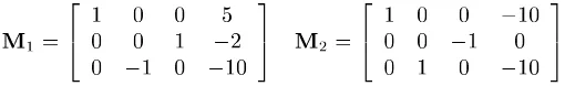
. We define two camera matrices:
✟
The reconstruction of the curve from the two projections has been made in the point space, using FGb1, a power-ful software tool for Gr¨obner basis computation [8, 9]. As expected there are two irreducible components. One has de-gree✼ and is the original curve, while the second has degree
✠ ✝
.
For the next experiment, we consider seven images of an electric wire — one of the views is shown in figure 2. In each image, we perform segmentation and thinning of the image curve. Hence for each of the images, we extracted a set of points lying on the thread. No fitting is performed in the image space. For each image, the camera matrix is cal-culated using the calibration pattern. Then we proceeded to compute the Chow polynomial of the curve in space. The curve has degree✓
. Once is computed, a reprojection is easily performed, as shown in figure 3.
5. Conclusion
In this paper we have focused on general (non-planar) al-gebraic curves as the building blocks from which the cam-era geometries are to be recovered and as the scene build-ing blocks for the purpose of reconstruction from multiple views. The new results derived in this paper include:
1Logiciel conc¸u et r´ealis´e au laboratoire LIP6 de l’universit´e Pierre et
Figure 3. Reprojection on a new image.
1. Extended Kruppa’s equations for the recovery of epipolar geometry from two projections of algebraic curves.
2. Dimension analysis for the minimal number of albraic curves required for a solution of the epipolar ge-ometry.
3. Reconstruction from two views of a curve of degree
✄
is a curve which contains two irreducible components one of degree
✄
and the other of degree
✄✆☎✝✄ ✞ ✠☞☛
— a result that leads to a unique reconstruction of the orig-inal curve.
4. Formula for the minimal number of views required for the reconstruction of the dual curve.
5. Formula for the minimal number of views required for the reconstruction of the curve representation✣
☎ ✠✜✓
✓
☛
.
Acknowledgment
We express our gratitude to Jean-Charles Faugere for giving us access to his powerful systemFGb. This research is partially sup-ported by the Emmy Noether Research Institute for Mathematics and the Minerva Foundation of Germany and the excellency center (Group Theoretic Method In The Study Of Algebraic Varieties) of the Israeli Academy of Science.
References
[1] J.Y.Kaminski Multiple-view Geometry of Algebraic Curves. Phd dissertation, submitted to Hebrew University of Jerusalem, May. 2001.
[2] K. Astrom and F. Kahl. Motion Estimation in Image Se-quences Using the Deformation of Apparent Contours. In
IEEE Transactions on Pattern Analysis and Machine Intelli-gence, 21(2), February 1999.
[3] R. Berthilson, K. Astrom and A. Heyden. Reconstruction of curves in✂✁, using Factorization and Bundle Adjustment. In
IEEE Transactions on Pattern Analysis and Machine Intelli-gence, 21(2), February 1999.
[4] D. Eisenbud. Commutative Algebra with a view toward alge-braic geometry. Springer-Verlag, 1995.
[5] D. Eisenbud and J. Harris. The Geometry of Schemes. Springer-Verlag, 2000.
[6] O.D. Faugeras Three-Dimensional Computer Vision, A geo-metric approach. MIT Press, 1993.
[7] 0.D. Faugeras and T. Papadopoulo. Grassman-Cayley algebra for modeling systems of cameras and the algebraic equations of the manifold of trifocal tensors. Technical Report - INRIA 3225, July 1997.
[8] J.C. Faugere. Computing Grobner basis without reduction to zero (✄✆☎). Technical report, LIP6, 1998.
[9] J.C. Faugere. A new efficient algorithm for computing Grob-ner basis (✄✞✝ ).
[10] D. Forsyth, Recognizing algebraic surfaces from their out-lines.
[11] Quadric Reconstruction from Dual-Space Geometry, 1998.
[12] J. Harris Algebraic Geometry, a first course. Springer-Verlag, 1992.
[13] Multiple View Geometry in computer vision. Cambridge Univeristy Press, 2000.
[14] R. Hartshorne. Algebraic Geometry. Springer-Verlag, 1977.
[15] F. Kahl and A. Heyden. Using Conic Correspondence in Two Images to Estimate the Epipolar Geometry. InProceedings of the International Conference on Computer Vision, 1998.
[16] J.Y. Kaminski and A. Shashua. On Calibration and Recon-struction from Planar Curves. InProceedings European Con-ference on Computer Vision, 2000.
[17] Q.T Luong and T. Vieville. Canonic Representations for the Geometries of Multiple Projective Views. InProceedings Eu-ropean Conference on Computer Vision, 1994.
[18] S.D. Ma and X. Chen. Quadric Reconstruction from its Oc-cluding Contours. InProceedings International Conference of Pattern Recognition, 1994.
[19] S.D. Ma and L. Li. Ellipsoid Reconstruction from Three Perspective Views. InProceedings International Conference of Pattern Recognition, 1996.
[20] S.J. Maybank and O.D. Faugeras A theory of self-calibration of a moving camera. International Journal of Computer Vi-sion, 8(2):123–151, 1992.
[21] T. Papadopoulo and O. Faugeras Computing structure and motion of general 3d curves from monocular sequences of perspective images. InProceedings European Conference on Computer Vision, 1996.
[22] T. Papadopoulo and O. Faugeras Computing structure and motion of general 3d curves from monocular sequences of per-spective images. Technical Report 2765, INRIA, 1995.
[23] L. Quan. Conic Reconstruction and Correspondence from Two Views. InIEEE Transactions on Pattern Analysis and Machine Intelligence, 18(2), February 1996.
[24] C. Schmid and A. Zisserman. The Geometry and Matching of Curves in Multiple Views. InProceedings European Con-ference on Computer Vision, 1998.