commit to user
CAPITAL ASSET PRICING MODEL (CAPM): THE THEORY AND EVIDENCE IN INDONESIA STOCK EXCHANGE (IDX) AT THE PERIOD
2004-2009
To Meet The Requirements of Master Degree Achievement from
Magister Management Study Program
Main interest:
Financial Management
Proposed by :
Arum Setyowati NIM: S4108008
MAGISTER MANAGEMENT STUDY PROGRAM POST GRADUATE PROGRAM
commit to user
CAPITAL ASSET PRICING MODEL (CAPM): THE THEORY AND EVIDENCE IN INDONESIA STOCK EXCHANGE (IDX)
AT THE PERIOD 2004-2009
Proposed by :
Arum Setyowati NIM: S4108008
Advisors approved
04th October 2010
Advisor I
Prof. Dr. Hartono, MS NIP. 130814578
Advisor II
Endang Suhari, S.E, M.Si NIP. 131570303
Approved by:
Director of Magister Management Study Program
commit to user
CAPITAL ASSET PRICING MODEL (CAPM): THE THEORY AND EVIDENCE IN INDONESIA STOCK EXCHANGE (IDX)
AT THE PERIOD 2004-2009
Proposed by :
Arum Setyowati NIM 4108008
Approved by the Examiners Team
On November 5th 2010
Examiners Team Leader : Dr. Bandi, M.Si, Ak ………
Advisor I : Prof. Dr. Hartono, MS ………
Advisor II : Dra. Endang Suhari, M.Si ………
Known by
Director of PPs UNS
Prof. Dr. Suranto, M. Sc. Ph.D NIP. 131 472 192
Director of Magister Management Program
commit to user
DECLARATION
Name: Arum Setyowati
NIM: S4108008
Stating that the thesis entitled CAPITAL ASSET PRICING MODEL (CAPM): THE THEORY AND EVIDENCE IN INDONESIA STOCK EXCHANGE (IDX) AT THE PERIODE 2004-2009 is my work. Things that are not my work in this thesis are marked citasi and shown in the bibliography.
If at a later date proved that my statement was not true, I am willing to receive
academic sanctions such as revocation of a degree thesis.
Surakarta, September 2010
commit to user
PREFACE
All praise to Allah SWT for all the abundance and his grace so that the
preparation of the thesis with the title "Capital Asset Pricing Model (CAPM): The
Theory and Evidence in Indonesia Stock Exchange (IDX) at the Period of
2004-2009" has been successfully finished. This thesis examines the validity of CAPM
theory by taking the object of research in Indonesia Stock Exchange (IDX).
In the preparation process of this report, the authors obtained a lot of instructions,
guidance and support from various parties. Therefore, with all humility, I say thank
you to:
1. Prof. Dr. Bambang Sutopo, M. Com, Ak. as Dean of the Faculty of
Economics, Sebelas Maret University.
2. Prof. Dr. Hartono, MS as Director of Magister Management Study Program
and Advisor I that have been patiently providing guidance and suggestions in
writing this essay.
3. Dra. Endang Suhari, M.Sc., as Advisors II that has been giving a lot of input
in the writing of this thesis.
4. My beloved father and mother who has given me a lot of sacrifices, and
special for my sister with all your affection.
commit to user
6. All parties who can not mention one by one author who has helped many
writers in preparing this paper.
I realize that the writing of this report is far from perfect. To the authors are
looking forward to critiques and suggestions for improvement and perfection of this
simple masterpiece. Finally, I hope that this modest work can be beneficial to all
parties.
commit to user
CONTENTS
CHAPTER I (INTRODUCTION) ………..
A. Background ……….
B. Problems ……….
C. Objectives ………...
CHAPTER II (THEORITICAL FRAMEWORK) ………
A. Return ……….
1. Realized Return ………
2. The Expected Return ………
3. Market Return ………..
B. Risk ……….
1. Portfolio Risk ………
2. Market Risk ………..
3. Risk Free Asset ……….
4. The Components of portfolio Risk (Correlation and Variance) …...
C. Capital Asset Pricing Model ………...
1. CAPM Assumption ………..
2. The Capital Market Line ………..
3. The Concept of Beta ……….………
commit to user
5. Research Framework ……….………...
5.1. Framework ……….………
5.2. Hypothesis ………..……...
CHAPTER III (DESCRIPTION OF DATA AND METHODOLOGY) ……...
A. Research Method ………
B. The Method of Data Collection ………..
C. Analysis Method ……….
CHAPTER IV (THE RESULT) ……….
Realized return ………..
Risk Free Asset ……….
Market Risk ………..
Equation 1 ……….
Equation 2 ……….
Equation 3 ……….
Equation 4 ……….
CHAPTER V (CONCLUSION) ……….
Conclusion …………..………..
commit to user
ABSTRACT
This research aims to examine the validity of the CAPM that was developed by Sharpe [1964], Litner [1965], and Mossin [1966] for all of the stock in Indonesia Stock Index (IDX). The study uses monthly stock returns from 213 companies listed on the Indonesia stock Exchange, certificate of Bank
Indonesia asrf, and stock price index for seek rm.
The sample of this thesis is enterprise who listed in Indonesia Stock Exchange at the period 2004 – 2009 and I got 213 samples. The findings of this research are not supported the theory’s basic statement that higher risk (beta) is associated with higher levels of return. The CAPM’s prediction for the intercept is that it should equal zero, the results of the study refute the above hypothesis and offer evidence against the CAPM theory.
commit to user
CHAPTER I
INTRODUCTION
A. Background
Capital market is a long-term investment alternative for the investors.
Each investment option has a rate of return and different risk. In fact, the
return and risk of stocks would differ even within the same industry. This is
caused by the different internal factors (management, marketing, financial
condition, product quality and competitive ability) and external factors
(government policy, competitors, and the taste and purchasing power of
people).
Based on the data from website Indonesia Stock Exchange (IDX), the
capital market in Indonesia has actually existed long before the Independence
of Indonesia. The first stock exchange in Indonesia was established on 1912
in Batavia during the Dutch colonial era. At that time, the Exchange was
established for the interest of the Dutch East Indies (VOC). During those eras,
the capital market grew gradually, and even became inactive for a period of
time due to various conditions, such as the World War I and II, power
transition from the Dutch government to Indonesian government, etc.
Indonesian government reactivated its capital market in 1977, and it grew
rapidly ever since, along with the support of incentives and regulations issued
commit to user
As an investment tool, capital market can be utilized for the investors
to invest their funds and increase investment choices. As a result of the many
investment choices offered, of course, investors need some considerations
such as financial information, computation and analysis of sufficient and need
to understand the situation and prospects of companies whose sell their stock
in the capital market. In deciding to invest their stock, investors should be
more selective in choosing stocks return. First, investors must estimate the
risks and the advantages to be gained or estimate the expected return is
greater than the realize return is not good to buy. Because it shows that it can
not meet the expectations of investors. Thus, a good stock to buy is stocks
with realized return greater than the expected return.
Many strategies and methods that can be used to estimate the return of
a security, it can be determined what level of benefits and risk of the
stock. Capital Asset Pricing Model (CAPM) is one of the many theories that
explain the relationship between risks and return level. Andre F [2004] said
that a fundamental question in finance is how the risk of an investment should
affect its expected return. The Capital Asset Pricing Model (CAPM) provided
the first coherent framework for answering this question. The CAPM is based
on the idea that not all risks should affect asset prices. In particular, a risk that
can be diversified away when held along with other investments in a portfolio
is, in a very real way, not a risk at all. The CAPM gives us insights about
commit to user
CAPM theory developed by Sharpe [1964], Litner [1965], and Mossin
[1966] became a major model used in the discussion of financial management
to estimate the return based on its risk. CAPM suggests that high expected
returns are associated with high levels of risk. Simply stated, CAPM
postulates that the expected return on an asset above the risk-free rate is
linearly related to the systematic risk/ market risk as measured by the asset’s
beta. Unsystematic risk or unique risk of each asset is assumed can be
eliminated with diversification.
Many empirical studies conducted to test the validity of the CAPM
model. Black, Jensen and Scholes [1972], using monthly return data tested
whether the cross-section of expected returns is linear in beta. The author
found that the relation between the average return and beta is very close to
linear and that portfolios with high (low) betas have high (low) average
returns. Fama and MacBeth [1973] examined that there is a positive linear
relation between average returns and beta. They investigated that the squared
value of beta and the volatility of asset returns can explain the residual
variation in average returns across assets that are not explained by beta alone.
While unsystematic risk or unique risk of each asset is assumed to be
eliminated because diversify.
Then some other researcher goes to measure the validity of CAPM
model by Sharpe [1964], Litner [1965], dan Mossin [1966]. Banz [1981], he
tested the CAPM by checking whether the size of firms can explain the
commit to user
the CAPM’s beta. He concluded that the average returns on stocks of small
firms (those with low market values of equity) were higher than the average
returns on stocks of large firms (those with high market values of equity).
This finding has become known as the size effect.
Other researchers are Fama and French [1992]. They used the same
procedure as Fama and McBeth [1973] but arrived at very different
conclusions. Fama and McBeth find a positive relation between return and
risk while Fama and French find no relation at all. While, Pettengill,
Sundaram and Mathur (1995) with different method found based on
estimation conditional on the signs of the market excess returns indicate that
betas and returns are positively related in the US capital market.
Fama and French [2004] said the capital asset pricing model (CAPM)
is still widely used in applications, such as estimating the cost of capital for
firms and evaluating the performance of managed portfolios. It is the
centerpiece of MBA investment courses. Indeed, it is often the only asset
pricing model taught in these courses. The attraction of the CAPM is that it
offers powerful and intuitively pleasing predictions about how to measure
risk and the relation between expected return and risk. Unfortunately, the
empirical record of the model is poor-poor enough to invalidate the way it is
used in applications.
Zhang and Wihlborg [2004] said that Capital Asset Pricing Model
(CAPM) developed by Sharpe (1964), Lintner (1965) and Mossin (1966) can
commit to user
and to estimate the cost of equity capital is an issue receiving attention only
recently. Since each emerging market has its own unique market structure,
institutional background, history, level of the market integration, and local
risk-free return, the answer may differ across countries. Moreover, whether
the CAPM is an appropriate model to the asset pricing in developed markets
is still controversial. In theory, beta as a single systematic risk measure has
been challenged by the alternative equilibrium asset-pricing model, the
Arbitrage Pricing Theory (APT).
Pettengill et al. (1995) propose a different methodology to estimate
the relationship between betas and returns. Their argument is that since the
CAPM is estimated with realized returns as proxies for expected returns, it is
likely that negative realized premium risk will be observed in some periods.
The model of Pettengill et al. is conditional on the realized risk premium,
whether it is positive or negative. When the realized risk premium is positive,
there should be a positive relationship between the beta and return, and when
the premium is negative, the beta and return should be negatively related. The
reason is that high beta stocks will be more sensitive to the negative realized
risk premium and have a lower return than low beta stocks.
The last, Michailidis, Tsopoglou, Papanastasiou [2006] measured
validity of CAPM model and the result are not supported the theory’s basic
CAPM model. The higher risk (beta) is not associated with higher levels of
commit to user
returns on the market portfolio. And residual risk has no effect on the
expected returns of portfolios.
This thesis will reexamine validity of CAPM model by Sharpe [1964],
Litner [1965], dan Mossin [1966] in the capital market of Indonesia. The
samples that used are the companies listed in Indonesia Stock Exchange
(IDX) during the period 2004-2009. Therefore this research takes the title:
CAPITAL ASSET PRICING MODEL (CAPM): THE THEORY AND
EVIDENCE IN INDONESIA STOCK EXCHANGE (IDX) AT THE
PERIOD 2004 - 2009.
B. Problems
Based on previous research about the validity of CAPM theory, I will
reexamine the validity of CAPM theory with Indonesia Capital Market as
sample. The research question that can be formulated are:
1. There is a positive linear relationship between the stock’s expected
returns and its systematic risk (beta). Does higher risk (beta) associate
with a higher level of return?
2. Based on the CAPM model with use method from Fama and MacBeth
(1973), is the intercept (expected excess return on a zero beta portfolio) is
commit to user
3. Based on the CAPM model with by using the method from Fama and
MacBeth (1973), is the intercept of risk premium significantly
positive?
4. Based on CAPM model by using the method from Pettengill et al. [1995],
is the intercept of premium risk significantly positive ( when up
market (excess return is positive)?
5. Based on CAPM model, by using the method from Pettengill et al. (1995),
is the intercept of premium risk significantly negative ( when
down market (excess return is negative)?
C. Objectives
The purpose of this study is to re-test the validity of CAPM model. Is
the CAPM model developed by Sharpe [1964], Litner [1965], and Mossin
[1966] still consistent in case capital market in Indonesia? This research will
prove empirically from the problems and previous findings that is:
1. To know whether there is or there isn’t a positive linear relationship
between the stock’s expected returns and its systematic risk (beta) and the
higher risk (beta) associate with a higher level of return.
2. To know whether intercept (expected excess return on a zero beta
portfolio) is equal to zero or not based on the CAPM model by using the
commit to user
3. To know whether the intercept of premium risk is significantly
positive or not based on the CAPM model by using the method from
Fama and MacBeth (1973).
4. To know whether the intercept of premium risk is significantly positive
( when up market (excess return is positive) based on CAPM
model by using the method from Pettengill et al. (1995).
5. To know whether the intercept of premium risk is significantly negative
( when down market (excess return is negative) based on CAPM
commit to user
CHAPTER II
THEORITICAL FRAMEWORK
A. Return
Return can be a realized return has happened and the expected return
that have not happened, but is expected to occur in the future. In measure
return, the realization of widely used measurement of total return, this is the
overall return from an investment in a period. The calculation of return is also
based on historical data. This realized return can be used as one measure of
company performance and can be as basic determinants of return expectations
and risk in future (Brigham and Daves, 2004).
Otherwise, expected return is return that be expected will be earned by
investors in the future. Thus, the difference between the two is the realization
of its returns has already happened, while the return expectation of it’s yet to
happen. Jogianto [1998] suggested that the return as a result can be obtained
from the investment return and the realization of expected return.
1. Realized return ( )
Brigham and Daves [2004] said that realized return is the return
that has occurred and is calculated based on historical data. Return the
commit to user
performance as well as the basis for determining the risk and expected
return in the future. One type of measurement that is often used
realization of return is total return, ie the overall return from an
investment in a given period.
= realized return at ‘i’ enterprise
= stock price at t period
= stock price at t-1 period
2. The expected return ( )
Brigham and Daves [2004] said that he very important principle
that should always be kept in the mind is “regardless of the number of
assets held in a portfolio, or the proportion of total investable funds
placed in each asset, the expected return on the portfolio is always a
weighted average of the expected returns for individual assets in the
portfolio.”
The percentage of portfolio’s total value that are invested in each
portfolio asset are referred to as portfolio weights, which we will denote
commit to user
percent of total investable funds or 1.0, indicating that all portfolio funds
are invested, that is:
If we multiply each possible outcome by its probability of
occurrence and then sum the products, we have a weighted average of
outcomes. The weights are the probabilities, and the weighted average is
expected return, . The expected rate of return calculation can also be
expressed as an equation:
= is the expected return
= the probability of the ith outcome
= 1.0
= is the ith possible outcome
commit to user
We can call also “market portfolio”. It is required rate of return
portfolio consisting of all stocks. It is also the required rate of return on an
average (β = 1) stock (Brigham and Daves, 2004).
B. Risk
1. Portfolio Risk
Risk is defined as the uncertainty about the actual return that
will be earned on an investment (John, 2007). The remaining
computation in investment analysis is that of the risk of the
portfolio. Brigham and Daves [2004] measure portfolio risk by the
standard deviation of its return with probability distribution. One
such measure is the standard deviation, the symbol for which is σ,
pronounced “sigma”. The smaller the standard deviation, the tighter
the probability distribution, and accordingly the less risky the stock.
To calculate the standard deviation, we taking step:
a.Calculate expected return:
b. Subtract the expected rate of return from each possible
commit to user
c.Square each deviation, then multiply the result by the probability
of occurrence for its related outcome:
d. Finally, find the square root of the variance to obtain the
standard deviation:
Where is the portfolio’s standard deviation; is the
return on in the ith state of the economy; is the expected
rate of return; is the probability of occurrence of the ith state
of the economy; and there are n economic states.
When the data aren’t in the form of a known probability
distribution, and if only sample returns data over some past
period are available, the standard deviation of returns can be
commit to user
Unlike return, the risk portfolio, σp, is generally not the
weighted average of the standard deviations of the individual
assets in the portfolio. The portfolio risk will almost always be
smaller than weighted average of the asset’s σ’s. In fact, it is
theoretically possible to combine stocks that are individually
quite risky as measured by their standard deviations to form a
portfolio that is completely risk, with σp = 0.
For example, stocks W and M can be combined to form a
riskless portfolio is that their return move counter cyclically to
each other when W’s returns fall, those of M rise, and vice
versa. The tendency of two variables to move together is called
‘correlation’, and the correlation coefficients measure this
tendency. The symbol for the correlation coefficient is ρ
(pronounced ‘roe’). In statistical terms, we say that the returns
on stocks W and M are perfectly negatively correlated, with ρ =
-1,0.
The opposite, it is perfect positive correlation, with ρ =
+1,0, when the returns M and W are move up and down
together, and a portfolio consisting of two such stocks would be
exactly as risky as each individual stock.
commit to user
Market risk is stems from factors that systematically affect most
firms: war, inflation, recessions, and high interest rate. Since most
stocks are negatively affected by these factors, market risk can not be
eliminated by diversification (Daves and Bringham, 2004).
3. Risk Free Rate ( )
Brigham and Daves [2004] said that the one assumption of
capital market theory is that investors can borrow and lend at the risk
free rate. Investors can invest part of their wealth in this asset and the
remainder in any of the risky portfolios in the Markowitz efficient set.
This allows Markowitz portfolio theory to be extended in such away
that the efficient frontier is completely changed, which in turn leads to a
general theory for pricing assets under uncertainty.
The risk free asset can be defined as one with a
certain-to-be-earned expected return and variance of return of zero. Since variance =
0, the nominal risk free rate in each period will be equal to its expected
value. Furthermore, the covariance between the risk free assets and the
any risky asset i will be zero (Jones, 2007).
4. The Components of portfolio Risk (Correlation and Variance)
commit to user
Daves and Brigham [2004] said that two key concepts in
portfolio analysis are covariance and the correlation coefficient.
a. Weighted individual security risk (i.e., the variance of each
individual security, weighted by the percentage of investable funds
placed in each individual security).
b. Weighted comovements between securities return (i.e., the
covariance between the securities returns, again weighted by the
percentage of investable funds placed in each security).
Covariance is a measure that combines the variance (or
volatility) of stock’s return with the tendency of those returns to move
up or down at the same time other stocks move up or down. This
equation defines the covariance between stocks A and B.
Where:
= the covariance between securities A and B
= one possible return on security A
= the expected value of the return on security A
= the number of likely outcomes for a security for the period
commit to user
When the data aren’t in the form of a known probability
distribution, and if only sample returns data over some past period are
available, the covariance of returns can be estimated using this formula:
Correlation coefficient
It is difficult to interpret the magnitude of the covariance term,
so a related statistic, the correlation coefficient, is generally used to
measure the degree of co movement between two variables. The
correlation coefficient standardizes the covariance by dividing by a
product term, which facilitates comparisons by putting things on a
similar scale. The correlation coefficient, ρ, is calculated as follows for
variables A and B.
It measures the extent to which the return on any two securities
is related; however, it denotes only association that is bounded by +1.0
and -1.0 with:
commit to user
The return has a perfect direct linier relationship. When the
returns are perfectly positively correlated, the risk of a portfolio is
simply weighted average of the individual risk of the securities.
= -1.0 (perfect negative/ inverse correlation)
In a perfect negative correlation, the securities returns have a
perfect inverse linier relationship to each other. Therefore, knowing the
return on one security provides full knowledge about the return on the
second security. When one security’s return is high, the other is low.
= 1.0 zero correlation
If the correlation is zero, there is no linier relationship between
the returns on the two securities. Combining two securities with zero
correlation (statistical independence) with each other reduces the risk of
portfolio.
Relating the correlation coefficient and the covariance
The variance and the correlation coefficient can be related in the
following manner:
commit to user
The two asset case
Under the assumption that the distributions of returns on the
individual securities are normal, a complicated looking but
operationally simple equation can be used to determine the risk of a
two-asset portfolio.
C. Capital Asset Pricing Model
The CAPM builds on the model of portfolio choice developed by
Harry Markowitz [1959]. In Markowitz's model, an investor selects a
portfolio at time t-1 that produces a stochastic return at t. The model assumes
investors are risk averse and, when choosing among portfolios, they care only
about the mean and variance of their one-period investment return. As a
result, investors choose "mean-variance-efficient" portfolios, in the sense that
the portfolios 1) minimize the variance of portfolio return, given expected
return, and 2) maximize expected return, given variance. Thus, the Markowitz
commit to user
Capital asset pricing model is an important tool to analyze the
relationship between risk and rates of return. The primary conclusion of the
CAPM is this: the relevant risk of an individual stock is its contribution to the
risk of a well-diversified portfolio.
The model was developed to explain the differences in the risk
premium across assets. According to the theory these differences are due to
differences in the riskiness of the returns on the assets. The model states that
the correct measure of the riskiness of an asset is its beta and that the risk
premium per unit of riskiness is the same across all assets. Given the risk free
rate and the beta of an asset, the CAPM predicts the expected risk premium
for an asset (Michailidis, et al., 2006).
1. CAPM Assumption
Brigham and Daves [2004] said that the CAPM is often
criticized as being unrealistic because of the assumptions on which it is
based, so it is important to be aware of these assumptions and the
reasons why they are criticized. The assumptions are as follows:
a. All investors focus on a single holding period, and they seek to
maximize the expected utility of their terminal wealth by choosing
among alternative portfolios on the basis of each portfolio’s
commit to user
b. All investors can borrow or lend an unlimited amount at a given
risk-free rate of interest, rf, and there are no restrictions on short
sales of any asset.
c. All investors have identical estimates of the expected returns,
variances, and covariances among all assets; that is investors have
homogeneous expectations.
d. All assets are perfectly divisible and perfectly liquid (that is,
marketable at the going price).
e. There are no transactions costs.
f. There are no taxes.
g. All investors are price takers (that is, all investors assume that their
own buying and selling activity will not affect stock prices).
h. The quantities of all assets are given and fixed.
2. The Capital Market Line
This straight line, usually referred to as the Capital Market Line
(CML), depicts the equilibrium condition that prevail in the market for
efficient portfolios consisting of the optimal portfolio of risky asset and
the risk-free asset.
The CML is a straight line without the now-dominated
Markowitz frontier. We know that this line has an intercept of rf. if
investors are to invest in risky asset, they must be compensated for this
commit to user
risk free rate and the CML at point M is the amount of return expected
of bearing the risk of owning a portfolio of stock, that is, the excess
return above the risk free rate. At that point, the amount of risk for the
risky portfolio of stock is given by the horizontal dotted line between rf
and σm.
The slope of CML is the market price of risk for efficient
portfolio. It is also called the equilibrium market price of risk. It
indicates the additional return that the market demands of each
percentage increase in a portfolio risk, that is, in its standard deviation
of return.
commit to user
3. The Concept of Beta
Brigham and Daves [2004] said that the benchmark for a well
diversified stock portfolio is the market portfolio, which is a portfolio
containing all stocks. Therefore, the relevant risk of an individual stock,
which is called its beta coefficient, is defined under the CAPM as the
amount of risk that the stock contributes to the market portfolio. In the
literature on the CAPM, it is proved that the beta coefficient of the ith
stock, denoted by βi, can be found as follow:
Or we can explain:
Here, ρim, is the correlation between the ith stock’s return and the
return on the market, σi is the standard deviation of the ith stock’s
return, and σm is the standard deviation of the market’s return.
The model was developed in the early 1960’s by Sharpe [1964],
Lintner [1965] and Mossin [1966]. In its simple form, the CAPM
predicts that the expected return on an asset above the risk-free rate is
linearly related to the non-diversifiable risk, which is measured by the
commit to user
The linear relationship between the return required on an
investment (whether in stock market securities or in business
operations) and its systematic risk is represented by the CAPM formula:
Where :
= return required on financial asset i
= risk-free rate of return
= beta value for financial asset i
= average return on the capital market
4. Test of CAPM Model Validity
Zhang and Wihlborg [2004], the CAPM states that there is a
positive, linear relationship between the stock’s expected returns and its
systematic risk, beta, and that beta is a sufficient variable to explain
cross sectional stock returns. The empirical evidence from the
developed equity markets generally shows only a weak relationship
between betas and returns (Fama and French 1992).
The CAPM predicts a positive linear relation between risk and
expected return of a risky asset of the form :
commit to user
Next, based on the method of Fama and MacBeth [1973], beta
estimated by regression model:
2)
The is the return on stock i, is the rate of return on a
risk-free asset, is the rate of return on the market index is the estimate of
beta for the stock i , and is the corresponding random disturbance
term in the regression equation. Equation 1 could also be expressed
using excess return notation, where } and
{ (Michailidis, et al., 2006).
The unconditional relationship between the beta and return is
estimated as:
3)
Where the regressions model from Eq. (2) and Eq. (3), and
are first estimated by OLS. Then, they are averaged by the t,
respectively. The average value, or is tested whether they are
commit to user
(1973). Based on Eq. (2), should be equal to zero and should be
significantly positive for a positive risk premium.
Pettengill et al. [1995] in Zhang and Wihlborg [2004] propose a
different methodology to estimate the relationship between betas and
returns. Their argument is that since the CAPM is estimated with
realized returns as proxies for expected returns, it is likely that negative
realized risk premium will be observed in some periods. The model of
Pettengill et al. is conditional on the realized risk premium, whether it is
positive or negative. When the realized risk premium is positive, there
should be a positive relationship between the beta and return, and when
the premium is negative, the beta and return should be negatively
related. The reason is that high beta stocks will be more sensitive to the
negative realized risk premium and have a lower return than low beta
stocks. According to the methodology of Pettengill et al., the
conditional relationship between the beta and return is estimated as :
4)
Where D is the dummy variable that equals one (1) if the
realized premium is positive and zero (0) if it is negative, is the
estimated risk premium in the up market period (with positive risk
commit to user
period (with negative premium risk). The average values, , ,
are tested for whether they are significantly different from zero using
the same t-test of Fama and MacBeth (1973). Thus, the null hypotheses
can be tested , against , . Pettengill et al.
(1995) point out that in order to guarantee a positive risk and return
tradeoff, two conditions should be met: i) the average risk premium
should be positive, and ii) the distribution of the up market periods and
down market periods should be symmetric.
5. Research Framework
This thesis re-tests the validity of CAPM model by Sharpe [1964],
Lintner [1965] and Mossin [1966] by using sample of Indonesia Stock
Exchange (IDX). In the later period, many researchers tested the validity of
CAPM model. Black et al. [1972], found that the relation between the
average return and beta is very close to linear and the portfolios with high
(low) betas have high (low) average returns. Fama [1973], Black tried to
retest and they found that there was a positive linear relation between average
returns and beta. They investigated that the squared value of beta and the
volatility of asset returns can explain the residual variation in average returns
across assets which are not only explained by beta. While unsystematic risk
or unique risk of each asset is assumed to be eliminated because of diversify.
commit to user
[1973], they arrived at very different conclusions. There was not a positive
relation between return and risk.
Pettengill et al. [1995], with different method based on estimation,
found when the realized risk premium is positive, there should be a positive
relationship between the beta and return, and when the premium is negative,
the beta and return should be negatively related.
This research retested the CAPM model by Sharpe [1964], Lintner
[1965] and Mossin [1966], with the method ‘two pass regression’ that was
used by Fama and McBeth [1973] and the method used by Pettengill et al.
[1995].
Framework
commit to user
6. Hypothesis
This thesis is a research that will test the validity of CAPM model by
commit to user
a positive linear relationship between the stocks’s expected returns and its
systematic risk (β) and that beta is a sufficient variable to explain cross sectional
stock returns (Zhang and Wihlborg, 2004). CAPM suggests that high expected
returns are associated with high levels of risk (Michailidis et al., 2006). From this
theory, the author proposes hypothesis:
H1: There is not a positive linear relationship between the stock’s expected
returns and its systematic risk (beta).
The Sharpe - Lintner CAPM says that the expected value of an asset's
excess return (the asset's return minus the risk-free interest rate, ) is
completely explained by its expected CAPM risk premium (its beta times the
expected value of ). This implies that “Jensen's alpha”, the intercept term
in the time-series regression, is zero for each asset (Fama and French, 2004).
From this theory, the author proposes hypothesis:
H2: The intercept (expected excess return on a zero beta portfolio) is not equal to
zero based on CAPM model ( .
Fama and MacBetch [1973] said, based on CAPM model, in a market of
risk-averse investors, higher risk should be associated with higher expected
commit to user
H3: The intercept of remium risk ( is not significantly positive (
Pettengill et al. [1995] argue that when the realized risk premium is
positive, there should be a positively relationship between the beta and return,
while if the premium is negative, the beta and return should be negatively related
since high beta stocks will be more sensitive to the negative risk premium and
have a lower return than low beta stocks. Based on the validity test of CAPM
procedure, the author proposes hypothesis 4 and 5:
H4: The intercept of premium risk is not significantly positive ( when up
market (excess return is positive).
H5: The intercept of premium risk is not significantly negative ( when
commit to user
CHAPTER III
DESCRIPTION OF DATA AND METHODOLOGY
A. Research Method
This research is a case study research that has objective to retest the
validity of the theory of CAPM on the stock market in Indonesia with the
object of research all companies listed in Indonesia Stock Exchange and
qualified as a sample. The observation uses monthly data from December
2003 to December 2009.
B. The Method of Data Collection
Population is the entire group, event, or an interest which will be
investigated by researchers (Sekaran, 2000). The population in this study is
all companies listed in Indonesia Stock Exchange (IDX). Data of companies’
stock price and the market return are obtained from www.yahoofinance.com,
while the risk free asset for the data is obtained from the monthly publication
of Bank Indonesia on Bank Indonesia Online Library.
Sekaran [2000], sample is a subset of the population. In this study,
the sample is determined by purposive sampling method on the basis of
commit to user
1. Companies listed on the Indonesia Stock Exchange in December 2003
- December 2009.
2. The companies traded every month during the period December 2003
- December 2009.
3. The companies have an average positive return during the study
period.
Based on these criteria we get 213 enterprises for the sample. The
enterprises are in appendix.
C. Analysis Method
The aims of this thesis are to measure the CAPM theory and the
evidence in Indonesia capital market. For regression testing, this study uses
SPSS software version 16 to know the relationship between risk and return,
and also to know the value of intercept. The regression model uses Fama dan
MacBeth [1973] procedure “two pass regression”.
The first step is to estimate a beta coefficient for each stock using
monthly returns during the period of January 2004 to December 2009. The
beta is estimated by regressing each stock’s monthly returnagainst the market
index according to the following equation:
commit to user
The next step is to compute the average of portfolio excess returns of
stocks ( ) ordered according to their beta coefficient computed by Equation
1. Let,
Where, k is the number of stocks included in each portfolio, p is the
number of portfolio, and is the excess return on stocks that form each
portfolio comprised of k stocks each. The procedure used is by dividing all
samples to 10 portfolios, so the author gets 22/21 for each portfolio. By
forming portfolios, the spread in betas across portfolios is maximized so that
the effect of beta on return can be clearly examined. The most obvious way to
form portfolios is to rank stocks into portfolios by the true beta. But, all that is
available observes beta. Ranking into portfolios by observed beta would
introduce selection bias. Stocks with high-observed beta (in the highest
group) would be more likely to have a positive measurement error in
estimating beta. This would introduce a positive bias into beta for high-beta
portfolios and would introduce a negative bias into an estimate of the
intercept (Elton and Gruber [1995], p. 333 in Michailidis et al., 2006).
To find hypothesis 1, the first step is compare the relationship of beta
and the return on each portfolio and the second step see a scatter plot of
commit to user
The following equation is used to estimate portfolio betas:
2)
Where is the average excess portfolio return, is the calculated
portfolio beta. The study is continued by estimating the ex-post Security
Market Line (SML) by regressing the portfolio returns against the portfolio
betas obtained by Equation 3. The relation examined is the following:
3)
Where, is the average excess return on a portfolio p (the difference
between the return on the portfolio and the return on a risk-free asset); is
an estimate of beta of the portfolio p; is the market price of risk, the risk
premium for bearing one unit of beta risk; is the zero-beta rate, the
expected return on an asset which has a beta of zero, and is random
disturbance term in the regression equation.
Pettengill et al. (1995) argued that the CAPM models the expected
returns, yet, in empirical research the realized returns are used as proxies for
the expected ones. Realized returns on the market portfolio often fall below
commit to user
observed in some periods. They propose an alternative methodology to
estimate the relationship between betas and returns. Their model is
conditional on whether the realized risk premium is positive or negative.
When the realized risk premium is positive, there should be a positive
relationship between the beta and return, while when the premium is negative,
the beta and return should be negatively related since high beta stocks will be
more sensitive to the negative risk premium and have a lower return than low
beta stocks (Zhang and Wihlborg, 2004). According to the methodology of
Pettengill et al, the conditional relationship between the beta and return is
estimated as:
commit to user
CHAPTER IV
THE RESULT
The main objective of this research is to reexamine the validity of CAPM
model by Sharpe [1964], Litner [1965], and Mossin [1966]. This research uses
Fama and McBeth [1973] procedure. First step is to estimates a beta coefficient
for each stock using monthly returns during the period of December 2003 to
December 2009. For calculating beta we need to know the realized return, the
market return and the risk free rate.
Realized return
To calculate the stock return, we need the stock price at the end of
monthly period. This paper uses 213 sample companies listed in Indonesia Stock
Exchange during the period of 2004 - 2009. Table 4.1. shows the value of the
stock price 213 companies listed in Indonesia Stock Exchange during the years
2004 - 2009.
commit to user
Risk Free Asset ( )
One form of the financial instrument that can be invested in Indonesia and
has risk free is Certificate of Bank Indonesia (SBI). Certificates of Bank
Indonesia are issued by the government so it obtains assurance. Risk obtained
by investors when investing in this asset is 0 because the certificates are issued
and guaranteed by the government (Bank Indonesia), so the possibility of Bank
Indonesia is not able to pay interest on the certificates is very small. Return to be
received by the investors in accordance with the amount of the interest rate is set
by the government. To calculate the return from risk-free asset uses SBI interest
rate monthly. The following tables show the value in monthly SBI during the
period of 2004 - 2009. The value of monthly will be shown in table 4.1.
To calculate we must find the average interest rate of SBI
Market Risk ( )
The market risk can be represented by assessing the average Composite
commit to user
say whether the market in a state of bullish (up) or bearish (weak). This market
indicts to help investors as an analysis tool in the decision whether to invest in the
stock market or not. We can calculate the market return using the value of the
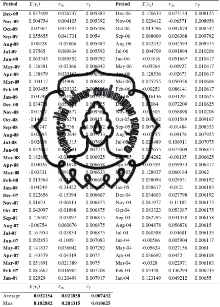
[image:48.595.114.470.242.502.2]stock price index (IHSG). The monthly Stock Price Index (IHSG) was shown in
table 4.1.
To calculate we must seek the average level of the Stock Price Index:
commit to user
Period ) Period )
Dec-09 0.037409 0.026737 0.005383 Dec-06 0.120633 0.075134 0.008125
Nov-09 0.004754 0.004105 0.005392 Nov-06 0.029412 -0.06571 0.008958
Oct-09 -0.02362 0.053403 0.005408 Oct-06 0.013296 0.097879 0.008542
Sep-09 0.055655 0.041731 0.0054 Sep-06 0.068069 0.026368 0.009792
Aug-09 -0.00428 -0.05866 0.005483 Aug-06 0.042432 0.042593 0.009375
Jul-09 0.07565 0.069834 0.005592 Jul-06 0.004709 0.091894 0.010208
Jun-09 0.063345 0.089552 0.005792 Jun-06 -0.01816 0.051667 0.010417
May-09 0.126381 -0.02366 0.006042 May-06 -0.05264 -0.00927 0.010417
Apr-09 0.138879 0.030162 0.006325 Apr-06 0.128536 -0.02673 0.010617
Mar-09 0.104117 0.04906 0.006842 Mar-06 0.055255 0.050356 0.010608
Feb-09 0.003455 0.020332 0.007283 Feb-06 -0.00253 0.086141 0.010617
Jan-09 -0.03798 -0.04048 0.007917 Jan-06 0.016136 0.031291 0.010625
Dec-08 0.034771 0.053832 0.009025 Dec-05 0.07064 0.072209 0.010625
Nov-08 -0.01327 0.007877 0.009367 Nov-05 -0.00505 0.058898 0.010208
Oct-08 -0.14662 0.146271 0.00915 Oct-05 0.008662 0.031589 0.009167
Sep-08 -0.09747 0.05736 0.008092 Sep-05 0.007098 -0.01484 0.008333
Aug-08 -0.02395 0.112644 0.007733 Aug-05 -0.07755 -0.09178 0.007925
Jul-08 -0.02608 0.201315 0.007692 Jul-05 0.021489 0.106911 0.007075
Jun-08 0.032887 0.115591 0.007275 Jun-05 0.022655 0.075009 0.006875
May-08 0.182882 -0.03541 0.006925 May-05 0.034282 -0.00135 0.006625
Apr-08 -0.04026 -0.01678 0.006658 Apr-05 -0.05359 0.059933 0.006417
Mar-08 -0.03331 0.091717 0.006633 Mar-05 0.128937 0.060184 0.0062
Feb-08 0.013364 -0.01206 0.006608 Feb-05 0.038094 0.028531 0.006192
Jan-08 -0.04249 -0.31422 0.006667 Jan-05 0.038617 -0.0121 0.006183
Dec-07 0.022656 -0.15394 0.006667 Dec-04 0.034603 0.027798 0.006192
Nov-07 0.01623 -0.06013 0.006875 Nov-04 0.081977 -0.11182 0.006175
Oct-07 0.043097 -0.01898 0.006875 Oct-04 0.083323 0.053387 0.006175
Sep-07 0.126302 -0.03897 0.006875 Sep-04 0.082795 0.031438 0.006158
Aug-07 -0.06754 0.060676 0.006875 Aug-04 0.004878 0.056876 0.00615
Jul-07 0.161954 -0.05834 0.006875 Jul-04 0.060588 -0.04681 0.006133
Jun-07 0.092853 -0.1009 0.007083 Jun-04 -0.00566 0.005904 0.006117
May-07 0.141837 0.036042 0.007292 May-04 -0.05624 0.027156 0.0061
Apr-07 0.143379 -0.04319 0.0075 Apr-04 0.036692 0.0452 0.006108
Mar-07 0.051891 0.021389 0.0075 Mar-04 -0.0328 0.022971 0.006183
Feb-07 0.081667 0.016962 0.007708 Feb-04 0.03448 0.136294 0.006233
Jan-07 0.02929 0.120498 0.007917 Jan-04 0.123149 0.049212 0.00655
)
Average 0.032154 0.021858 0.007432
Max 0.182882 0.201315 0.010625
Min -0.14662 -0.31422 0.005383
[image:50.595.109.545.112.721.2]commit to user
From the average value of and , we can see that the average value of
risk free asset is (0.7432%) par month. That is lower than the average value of
(market return) which amounted to 2.1858%. The difference between these two
values is at 1.4426%. This shows that investing in the period 2004-2009 in the
Indonesia Stock exchange would be more profitable than investing in certificate
of Bank Indonesia.
Equation 1
The first part of the methodology requires the estimation of betas for
individual stocks by using observations on rates of return for a sequence of dates.
Useful remarks can be derived from the results of this procedure, for the assets
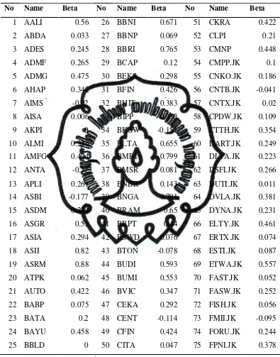
used in this study. The range of the estimated stock betas is between -0.92 the
commit to user
Table 4.2.
Stock beta coefficient estimates
No Name Beta No Name Beta No Name Beta
1 AALI 0.56 26 BBNI 0.671 51 CKRA 0.422
2 ABDA 0.033 27 BBNP 0.069 52 CLPI 0.21
3 ADES 0.245 28 BBRI 0.765 53 CMNP 0.448
4 ADMF 0.265 29 BCAP 0.12 54 CMPP.JK 0.1
5 ADMG 0.475 30 BEKS 0.298 55 CNKO.JK 0.186
6 AHAP 0.342 31 BFIN 0.426 56 CNTB.JK -0.041
7 AIMS -0.92 32 BHIT 0.383 57 CNTX.JK 0.02
8 AISA 0.006 33 BIPP 0.333 58 CPDW.JK 0.109
9 AKPI 0 34 BKSW -0.151 59 CTTH.JK 0.354
10 ALMI 0.276 35 BLTA 0.655 60 DART.JK 0.249
11 AMFG 0.494 36 BMRI 0.799 61 DLTA.JK 0.223
12 ANTA -0.32 37 BMSR 0.081 62 DSFI.JK 0.266
13 APLI 0.261 38 BNBR 0.143 63 DUTI.JK 0.011
14 ASBI -0.177 39 BNGA 0.701 64 DVLA.JK 0.381
15 ASDM 0.274 40 BRAM 0.65 65 DYNA.JK 0.231
16 ASGR 0.55 41 BRPT 0.44 66 ELTY.JK 0.461
17 ASIA 0.294 42 BSWD 0.076 67 ERTX.JK 0.074
18 ASII 0.82 43 BTON -0.078 68 ESTI.JK 0.087
19 ASRM 0.88 44 BUDI 0.593 69 ETWA.JK 0.557
20 ATPK 0.062 45 BUMI 0.553 70 FAST.JK 0.052
21 AUTO 0.422 46 BVIC 0.347 71 FASW.JK 0.252
22 BABP 0.075 47 CEKA 0.292 72 FISH.JK 0.056
23 BATA 0.2 48 CENT -0.114 73 FMII.JK -0.095
24 BAYU 0.458 49 CFIN 0.424 74 FORU.JK 0.244
25 BBLD 0 50 CITA 0.047 75 FPNI.JK 0.378
commit to user
Table 4.2 (continue)
Stock beta coefficient estimates
No Name Beta No Name Beta No Name Beta
76 GDYR 0.188 101 INTA 0.599 126 LSIP 0.616
77 GEMA 0.332 102 INTP 0.727 127 LTLS 0.285
78 GGRM 0.529 103 ITTG 0.129 128 MAMI 0.244
79 GJTL 0.666 104 JECC 0.152 129 MAYA -0.13
80 GMTD -0.236 105 JKSW 0.263 130 MBAI 0.3
81 GSMF 0.3 106 JPFA 0.367 131 MDLN 0.433
82 HERO 0.192 107 JPRS 0.412 132 MDRN 0.405
83 HEXA 0.407 108 KAEF 0.518 133 MEDC 0.585
84 HMSP 0.256 109 KARW 0.174 134 MEGA -0.006
85 IGAR 0.572 110 KBLI 0.534 135 MERK 0.573
86 IIKP 0.14 111 KBLM 0.042 136 MITI 0.34
87 IKAI 0.273 112 KDSI 0.492 137 MLBI 0.203
88 IKBI 0.252 113 KIJA 0.614 138 MLIA 0.428
89 IMAS 0.146 114 KLBF 0.546 139 MPPA 0.34
90 INAF 0.53 115 KPIG 0.151 140 MRAT 0.656
91 INAI 0.462 116 KREN 0.285 141 MREI 0.251
92 INCF -0.219 117 LAPD 0.61 142 MTDL 0.489
93 INCI 0.603 118 LION -0.141 143 MTFN 0.069
94 INDF 0.705 119 LMPI 0.308 144 MTSM 0.054
95 INDR 0.41 120 LMSH -0.068 145 MYOR 0.486
96 INDS 0.037 121 LPCK 0.277 146 NIPS 0.123
97 INDX 0.053 122 LPGI 0.187 147 NISP -0.096
98 INKP 0.456 123 LPIN 0.103 148 MORE -0.109
99 INPC 0.037 124 LPLI 0.068 149 PAFI -0.015
100 INRU 0.313 125 LPPS.JK 0.269 150 PANS.JK 0.365
[image:53.595.110.500.142.646.2]commit to user
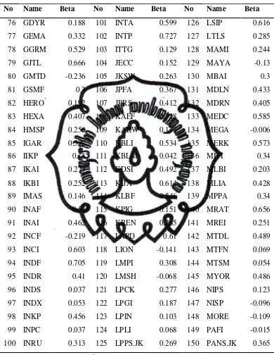
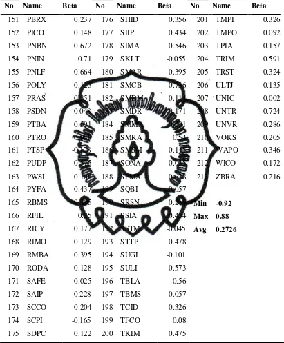
Table 4.2 (continue)
Stock beta coefficient estimates
No Name Beta No Name Beta No Name Beta
151 PBRX 0.237 176 SHID 0.356 201 TMPI 0.326
152 PICO 0.148 177 SIIP 0.434 202 TMPO 0.092
153 PNBN 0.672 178 SIMA 0.546 203 TPIA 0.157
154 PNIN 0.71 179 SKLT -0.055 204 TRIM 0.591
155 PNLF 0.664 180 SMAR 0.395 205 TRST 0.324
156 POLY 0.123 181 SMCB 0.736 206 ULTJ 0.135
157 PRAS 0.351 182 SMDM 0.114 207 UNIC 0.002
158 PSDN -0.048 183 SMDR 0.171 208 UNTR 0.724
159 PTBA 0.591 184 SMMA 0.291 209 UNVR 0.286
160 PTRO 0.088 185 SMRA 0.54 210 VOKS 0.205
161 PTSP -0.178 186 SMSM 0.115 211 WAPO 0.346
162 PUDP 0.575 187 SONA 0.035 212 WICO 0.172
163 PWSI 0.106 188 SPMA 0.628 213 ZBRA 0.216
164 PYFA 0.437 189 SQBI 0.057
165 RBMS 0.305 190 SRSN 0.215 Min -0.92
166 RFIL 0.25 191 SSIA 0.454 Max 0.88
167 RICY 0.177 192 SSTM -0.045 Avg 0.2726
168 RIMO 0.129 193 STTP 0.478
169 RMBA 0.395 194 SUGI -0.101
170 RODA 0.128 195 SULI 0.573
171 SAFE 0.025 196 TBLA 0.56
172 SAIP -0.228 197 TBMS 0.057
173 SCCO 0.204 198 TCID 0.326
174 SCPI -0.165 199 TFCO 0.08
175 SDPC 0.122 200 TKIM 0.475
[image:54.595.109.520.146.643.2]commit to user
Based on the table 4.1., it can be concluded that the 213 companies
sampled, all companies are the companies that have defensive stock because they
have the value (β < 1). The minimum value of beta in this sample is -0.92, the
maximum is 0.88 and the average is 0.2726.
Investors who are rational will choose the investment that is less risky if
they are faced with two investment options that provide the same return with a
different risk. Investors can assess the relationship between risk and return by
using the approach of Capital Assets Pricing Model (CAPM) to assess the
appropriate investment choices. Measurement of risk in the CAPM uses a β from
the previous calculation, while the return is measured by summing the risk-free
asset return with the excess of the average market return and return risk-free
asset. Difference in average market return and return risk-free asset is also called
the Risk Premium.
In order to diversify away most of the firm-specific part of returns,
thereby enhancing the precision of the beta estimates, the securities are
previously combined into portfolios. This approach mitigates the statistical
problems that arise from measurement errors in individual beta estimates. These
portfolios are created for several reasons: (i) the random influences on individual
stocks tend to be larger compared to those on suitably constructed portfolios
(hence, the intercept and beta are easier to estimate for portfolios) and (ii) the
tests for the intercept are easier to implement for portfolios because by
construction their estimated coefficients are less likely to be correlated with one
commit to user
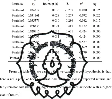
Equation 2
The article argues that certain hypotheses can be tested no matter of
whether one believes in the validity of the simple CAPM or in any other version
of the theory. Firstly, the theory indicates that higher risk (beta) is associated with
a higher level of return. However, the results of the study do not support this
hypothesis. The beta coefficients of the 10 portfolios do not indicate that higher
beta portfolios are related with higher returns. For example the portfolio 1 with
beta value -0.265 has return 0.034517 and portfolio 2 who has lower return
0.031161, in contras has higher beta 0.269. And portfolio 4 who has lower return
0.019933 than portfolio 2, it has higher beta value of portfolio 2 0.415. These
contradicting results can be partially explained by the significant fluctuations of
stock returns over the period examined (Table 4.3). The intercept in all of
commit to user
Table 4.3.
Average excess portfolio returns and betas
Portfolio intercept (α) Β sig.
Portfolio1 0.034517 0.038 -0.265 0.070 0.025
Portfolio2 0.031161 0.028 0.269 0.072 0.022
Portfolio3 0.035579 0.010 0.286 0.082 0.015
Portfolio4 0.028538 0.021 0.415 0.172 0.000
Portfolio5 0.020516 0.012 0.651 0.424 0.000
Portfolio6 0.023093 0.011 0.651 0.424 0.000
Portfolio7 0.019968 0.006 0.760 0.577 0.000
Portfolio8 0.019255 0.003 0.818 0.669 0.000
Portfolio9 0.014108 -0.003 0.883 0.779 0.000
Portfolio10 0.019178 0.003 0.882 0.779 0.000
From the table 4.3. we can say that we can not accept hypothesis, is that,
there is not a positive liner relationship between the stock’s expected returns and
its systematic risk (beta). The higher risk (beta) does not associate with a higher
level of return.
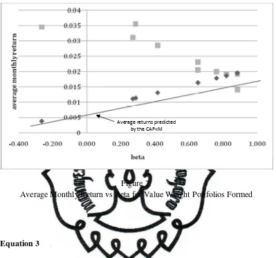
The Sharpe - Lintner CAPM predicts that the portfolios plot along a
straight line, with an intercept equal to the risk-free rate, , and a slope equal to
the expected excess return on the market, . We use the one-month
Certificate of Bank Indonesia rate and the market return of enterprises in
Indonesia Stock exchange for 2004 - 2009 to estimate the predicted line in figure
commit to user
Figure 2.
Average Monthly Return vs Beta for Value Weight Portfolios Formed
Equation 3
In order to test the CAPM hypothesis 2 and 3, it is necessary to find the
counterparts to the theoretical values that must be used in the CAPM equation. In
this study the Certificate of Bank Indonesia on the 1-month is used as an
approximation of the risk-free rate . For , the Composite Stock Index of
Indonesia Stock Exchange is taken as the best approximation for the market
portfolio.
The basic equation used is
commit to user
Where is the expected excess return on a zero beta portfolio and is
the market price of risk, the difference between the expected rate of return on the
market and a zero beta portfolio. This regression model was tested by Fama and
MacBeth (1973) model. Based on the CAPM theory should be equal to zero
and should be significantly positive for a positive risk premium.
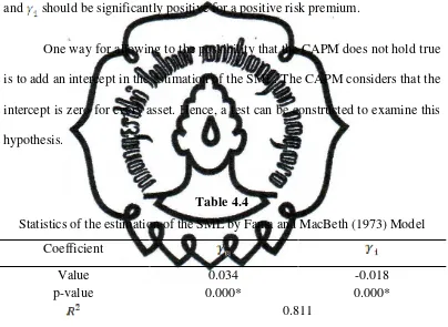
One way for allowing to the possibility that the CAPM does not hold true
is to add an intercept in the estimation of the SML. The CAPM considers that the
intercept is zero for every asset. Hence, a test can be constructed to examine this
[image:59.595.112.516.246.541.2]hypothesis.
Table 4.4
Statistics of the estimation of the SML by Fama and MacBeth (1973) Model
Coefficient
Value 0.034 -0.018
p-value 0.000* 0.000*
0.811
Source: Data are processed by SPSS
The results in table 4.4. indicate that the CAPM’s prediction for is that
it should be equal to zero. The calculated value of the intercept is small (0.034)
but it is not significantly different from zero (the p value is not greater than
commit to user
rejected. Based on CAPM model, intercept (expected excess return on a zero beta
portfolio) is not equal to zero.
According to CAPM the intercept of beta, (risk premium) should be
positive. The value of is -0.018 (negative), so we can conclude that based on
Fama and MacBeth (1973) model, we reject the hypothesis 3 that the intercept of
premium risk ( is not significantly positive ( .
From the hypothesis 2 and 3 we conclude that we can not accept the base
theory CAPM that intercept is equal to zero and premium risk is positive.
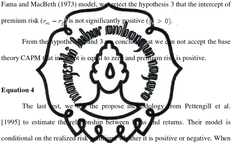
Equation 4
The last test, we test the propose methodology from Pettengill et al.
[1995] to estimate the relationship between betas and returns. Their model is
conditional on the realized risk premium, whether it is positive or negative. When
the realized risk premium is positive, there should be a positive relationship
between the beta and return, and when the premium is negative, the beta and
return should be negatively related. The reason is that high beta stocks will be
more sensitive to the negative realized risk premium and have a lower return than
[image:60.595.113.520.243.488.2]low beta stocks.
Table 4.5.
Statistics of the estimation of the SML by Pettengill et al. (1995) Model
commit to user
0.066 0.038
Value 0.134 -0.026
p-value 0.037 0.016
0.777
Sorce: Data are processed by SPSS
The results in table 4.5. indicate that the coefficients for (0.134) is
positive and these for (-0.026) is negative. All the coefficients are significant.
These results indicate that shares with higher betas have higher returns when the
local market excess return is positive and lower returns when the local market
excess return is negative. So, I can conclude that I can accept hypothesis 4 and 5,
based on CAPM model by Pettengill et al. (1995), intercept of premium risk is
significantly positive ( when up market (excess return is positive) with p
value 0.037, and intercept of premium risk is significantly negative (
when down market (excess return is negative) with p value 0.016. The intercept
commit to user
CHAPTER V
CONCLUSION
This thesis examines the validity of the CAPM for the all of stock in
Indonesia Stock Index (IDX). The study uses monthly stock returns from 213
companies listed on the Indonesia Stock Exchange from December 2003 to
December 2009. The data of return individual and stock price index for
measure market risk are obtained from www.yahoofinance.com. And for
variable risk free asset we use certificate of Bank Indonesia and get data from
library online of Bank Indonesia.
From the average value of and , we can see that the average value of
risk free asset (0.7432%) par month is lower than the average value of (market
return) which amounted to 2.1858%. The difference between these two values is
at 1.4426%. This shows that investing in the period 2004-2009 in the Indonesia
Stock exchange would be more profitable than investing in certificate of Bank
commit to user
Based on the result of the betas value from each enterprise, we can
conclude that the 213 companie