DEVELOPMENT OF A STATE PREDICTION MODEL TO AID DECISION MAKING IN CONDITION BASED MAINTENANCE.

DEVELOPMENT OF A STATE PREDICTION MODEL TO

AID DECISION MAKING IN CONDITION BASED

MAINTENANCE

B. HUSSIN

DEVELOPMENT OF A STATE PREDICTION MODEL TO

AID DECISION MAKING IN CONDITION BASED

MAINTENANCE

Burairah HUSSIN

Centre for Operational Research and Applied Statistics (CORAS)

University Of Salford, Salford UK

TABLES OF CONTENTS

TABLES OF CONTENTS ... I LIST OF FIGURES ... IV LIST OF TABLES ... VI NOTATIONS ...VIII ACKNOWLEDGMENTS ... IX ABSTRACT ... X

1 CHAPTER 1: INTRODUCTION ... 1

1.1 BACKGROUND AND MOTIVATION ... 1

1.2 ORGANIZATION OF THE THESIS ... 4

2 CHAPTER 2: LITERATURE REVIEWS ... 7

2.1 INTRODUCTION... 7

2.2 AN INTRODUCTION TO MAINTENANCE ... 7

2.3 CONDITION-BASED MAINTENANCE ... 11

2.4 COMPONENTS OF CONDITION-BASED MAINTENANCE ... 14

2.5 CONDITION-MONITORING TECHNIQUES... 17

2.5.1Vibration Monitoring ... 17

2.5.2 Oil Analysis ... 18

2.5.3 Temperature Monitoring... 19

2.6 DATA INTERPRETATION ... 19

2.7 CBMDECISION MAKING ... 20

2.8 MODELLING IN CONDITION-BASED MAINTENANCE ... 24

2.8.1 Proportional Hazards Model (PHM) ... 24

2.8.2 Proportional Intensities Model (PIM) ... 27

2.8.3 Markov Models ... 28

2.8.4 Stochastic Filtering... 30

2.9 COMPUTERIZED MAINTENANCE MANAGEMENT SYSTEMS... 34

2.10 SUMMARY ... 35

3 CHAPTER 3: FAULT PREDICTION USING CONDITION MONITORING INFORMATION ... 36

3.1 INTRODUCTION... 36

3.2 BACKGROUND OF HIDDEN MARKOV MODELS ... 37

3.3 MODELLING METHODOLOGY ... 39

3.4 FORMULATION OF THE TRANSITION PROBABILITIES ... 42

3.5 FORMULATION OF THE RELATIONSHIP BETWEEN THE OBSERVED DATA AND THE HIDDEN STATE ... 44

3.6 MODELLING DEVELOPMENT ... 44

3.7 NUMERICAL EXAMPLES ... 48

3.8 PARAMETER ESTIMATION ... 50

3.8.1 Maximum Likelihood Estimator ... 51

3.8.2 Expectation-Maximization (EM) Algorithm... 55

3.9 GOODNESS-OF–FIT TEST ... 58

4 CHAPTER 4: EARLY FAULT IDENTIFICATION – A CASE STUDY

USING VIBRATION DATA ... 64

4.1 INTRODUCTION... 64

4.2 NUMERICAL RESULTS ... 64

4.3 TESTING THE MODEL ... 67

4.4 COMPARISON WITH A STATISTICAL PROCESS CONTROL (SPC)CHART APPROACH ... 73

4.5 SUMMARY ... 75

5 CHAPTER 5: NUMERICAL APPROXIMATION TO FAULT PREDICTION TECHNIQUES ... 76

5.1 INTRODUCTION... 76

5.2 GRID-BASED METHOD ... 76

5.3 PARTICLE FILTER FOR A DISCRETE STATE CASE ... 81

5.3.1 Overview of the Particle Filtering Method ... 81

5.3.2 Implementation of Sequential Importance Sampling (SIS) for a Discrete Case ... 85

5.4 PARAMETER ESTIMATION ... 87

5.5 SUMMARY ... 90

6 CHAPTER 6: CONDITION BASED MAINTENANCE MODELLING BASED UPON OIL ANALYSIS DATA ... 91

6.1 INTRODUCTION... 91

6.2 BACKGROUND ... 92

6.3 DATA COLLECTION ... 92

6.3.1 Lifetime Data ... 93

6.3.2 Condition Indicators ... 93

6.3.3 Maintenance Events ... 93

6.4 DATA ANALYSIS ... 94

6.4.1 Principal Component Analysis ... 97

6.5 MODELLING METHODOLOGY ... 101

6.6 MODEL FORMULATION ... 102

6.7 PARAMETER ESTIMATION ... 107

6.8 THE CASE STUDY ... 111

6.9 CHECK THE GOODNESS-OF-FIT TO DATA ... 120

6.10 TESTING THE MODEL ... 124

6.11 THE DECISION MODEL... 128

6.12 SUMMARY ... 131

7 CHAPTER 7: CONDITIONAL RESIDUAL TIME MODELLING USING BOTH RESPONSIVE AND REFLECTIVE VARIABLES ... 132

7.1 INTRODUCTION... 132

7.2 MODEL DEVELOPMENTS ... 133

7.2.1 Notation... 133

7.2.2 Model Formulations ... 134

7.3 PARAMETER ESTIMATION ... 137

7.4 FITTING THE MODEL TO THE DATA ... 141

7.4.1 Independent Component Analysis (ICA) ... 142

7.5 MODEL COMPARISON ... 146

8 CHAPTER 8: A WEAR PREDICTION MODEL BASED ON

SPECTROMETRIC OIL ANALYSIS PROGRAMME USED IN DIESEL

ENGINES ... 148

8.1 INTRODUCTION... 148

8.2 MODELLING DEVELOPMENT ... 149

8.2.1 Notation... 149

8.2.2 Assumptions... 150

8.3 MODEL FORMULATION ... 150

8.4 MODEL APPROXIMATIONS ... 151

8.4.1 Approximated Grid Method ... 152

8.4.2 Particle Filtering ... 153

8.5 PARAMETER ESTIMATION ... 154

8.6 NUMERICAL RESULTS ... 156

8.7 SUMMARY ... 165

9 CHAPTER 9: CONCLUSION, DISCUSSION AND FUTURE RESEARCH ... 167

9.1 CONCLUSION OF THE RESEARCH ... 167

9.2 CONTRIBUTIONS OF THE RESEARCH ... 168

9.3 FUTURE RESEARCH AND OTHER ISSUES ... 170

REFERENCES ……….…………173

APPENDIX

LIST OF FIGURES

Figure 2-1: P-F curve ... 12

Figure 2-2: Detection of potential failures ... 13

Figure 2-3: Delay time concept ... 13

Figure 2-4: Hard and soft failures ... 16

Figure 2-5: Ilustration of pattern of the hazard function and the baseline hazard function. ... 25

Figure 2-6: Illustration of 3 states Markov model ... 29

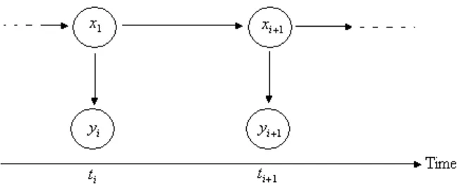
Figure 3-1: Graphical representation of the structure of a hidden Markov model ... 37

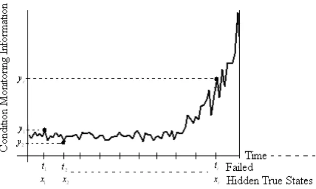
Figure 3-2: Processes of observation and hidden states ... 38

Figure 3-3: Two-stage failure process ... 40

Figure 3-4: Vibration data for six bearings ... 44

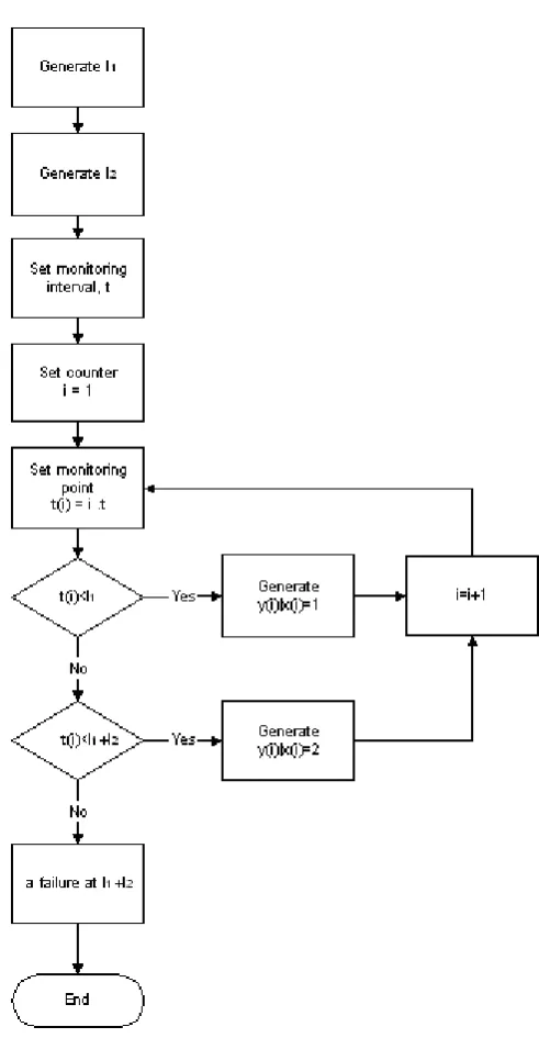
Figure 3-5: Set-up algorithm to generate simulated pattern data ... 46

Figure 3-6: Relationship between y_i and x_i ... 48

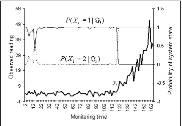
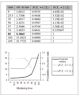
Figure 3-7: Case 1: Observed monitoring information and the probabilities of system state given _i ... 49

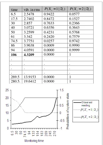
Figure 3-8: Case 2: Observed monitoring information and the probabilities of system state given i ... 49

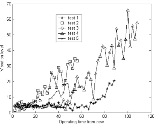
Figure 3-9: Simulation of five life cycles of data imitating the bearing case ... 52

Figure 3-10: The likelihood function at each monitoring point ... 53

Figure 3-11: Comparison between simulated, y~ , and observed values, y, for a particular case of simulated data ... 60

Figure 4-1: Case 1: Simulated and observed vibration levels for Gu-b3 ... 67

Figure 4-2: Case 2: Simulated and observed vibration levels for Gu-b4 ... 68

Figure 4-3: Partition the pdf of p(y_i|_i1) into equal probability and transform it to uniform distribution ... 70

Figure 5-1: Trellis diagram for grid-based filter ... 80

Figure 5-2: Identification of a random defect of bearing Gu-b3 using SIS algorithm (optimal density) ... 88

Figure 5-3: Identification of a random defect of bearing Gu-b3 using SIS algorithm (sub-optimal density) ... 89

Figure 6-1: Row format for monitoring data ... 94

Figure 6-2: Monitoring data after column manipulation ... 94

Figure 6-3: A sample of total metal concentration after the transformation ... 96

Figure 6-4: Case 1 – Choosing the dimensions of principal component analysis for engine 830001/19 ... 98

Figure 6-5: Case 2 – Choosing the dimensions of principal component analysis for engine 830001/26 ... 98

Figure 6-6: Re-organizing condition-monitoring data from original reading ... 100

Figure 6-7: The difference before and after re-organising ... 100

Figure 6-8: Examples of regular total metal concentration (1st PCA) used in diesel engine since new ... 101

Figure 6-9: Regression of total metal concentration and failure time ... 114

Figure 6-10: 95% prediction interval from regression of failure data ... 115

Figure 6-11: Typical monitoring observation ... 120

Figure 6-13: Case 2 – pdf and actual residual time with monitoring information for engine 830001/30 ... 122 Figure 6-14: pdf and actual residual time without monitoring information for engine

830001/28... 123 Figure 6-15: Case 1 – pdf of residual time of 830001/28 at last observation point ... 123 Figure 6-16: Case 2 – pdf of residual time of 830001/30 at last observation point ... 124 Figure 6-17: Partition the pdf of p(x_i|_i) into equal probability and transform to

uniform distribution ... 127 Figure 6-18: Case 1 – Expected cost per day in terms of planned replacement at time T

given that the current monitoring check is time t_i ... 130 Figure 6-19: Case 2 – Expected cost per day in terms of planned replacement at time T

given that the current monitoring check is time t_i ... 130 Figure 7-1: Case 1 – pdf and actual residual time with mixed monitoring information for engine 830001/28 ... 145 Figure 7-2: Case 2 – pdf and actual residual time with mixed monitoring information for engine 830001/30 ... 145 Figure 7-3: Case 1 – pdf residual time of engine 830001/28 at the last observation point

... 146 Figure 7-4: Case 2 – pdf residual time of engine 830001/30 at the last observation point

... 146 Figure 8-1: Algorithm for simulating a general beta distribution ... 160 Figure 8-2: Simulated and actual paths of monitoring information y_i for 901001/1 .. 161 Figure 8-3: Simulated and actual paths of monitoring information y_i for 830000/5 . 161 Figure 8-4: p(w_i) based on failure data only ... 163 Figure 8-5: p(w_i |_i) based on failure data and condition monitoring information of

LIST OF TABLES

Table 3-1: Simulation values ... 48

Table 3-2: The estimated parameters and their true values ... 53

Table 3-3: The estimated parameters and true values using the likelihood function with failure information ... 54

Table 3-4: The estimated parameters and true values Q(,j) ... 57

Table 3-5: The estimated parameters and true values with modified Q(,j) ... 58

Table 3-6: Variances and covariances of estimated parameters ... 59

Table 3-7: R2 for comparison between actual y_i and simulated y~_i ... 61

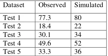
Table 3-8: The observed and simulated values for the initial time of a random defect .. 61

Table 4-1: Estimated parameters from vibration data... 64

Table 4-2: Variance and covariance matrix ... 65

Table 4-3: Case 1: P(x_i |_i)and the starting point of the abnormal stage for Gu-b3 ... 65

Table 4-4: Case 2: P(x_i |_i)and the starting point of the abnormal stage for Gu-b6 .. 66

Table 4-5: Values for Pearson product moment correlation coefficient ... 68

Table 4-6: Calculating the goodness-of-fit test ... 71

Table 4-7: E(L₁t_i,x_i |L₁t_i,_i) with exponential distribution for Gu-b3 ... 71

Table 4-8: E(L₁t_i,x_i |L₁t_i,_i)with Weibull distribution for Gu-b3 ... 72

Table 4-9: E(L₂ L₁t_i,x_i |L₂L₁ t_i,_i)with exponential distribution for Gu-b3 72 Table 4-10: E(L₂ L₁t_i,x_i |L₂L₁ t_i,_i) with Weibull distribution for Gu-b3 ... 73

Table 4-11: Starting point of the abnormal stage using SPC techniques and state prediction model ... 74

Table 5-1: Estimated parameters using the grid-based approach ... 87

Table 5-2: Estimated parameters using a particle filter with prior importance density .. 88

Table 5-3: Estimated parameters using a particle filter with optimal importance density ... 88

Table 6-1: Estimated parameters ... 112

Table 6-2: Variances of estimated parameters ... 112

Table 6-3: Estimated parameters for failure and interval-censored information ... 113

Table 6-4: Variances of estimated parameters for failure and interval-censored information ... 113

Table 6-5: Estimated parameters for 95 % prediction interval from regression of failure data... 116

Table 6-6: Variances of estimated parameters for 95 % prediction interval from regression of failure data ... 116

Table 6-7: Estimated parameters using interval-censored data ... 119

Table 6-8: Estimated parameters using anticipated data ... 119

Table 6-9: MSE of anticipated and interval data ... 119

Table 6-10: Variance and covariance results ... 120

Table 6-11: Calculating the confidence level ... 126

Table 6-12: Calculating the goodness-of-fit ... 128

Table 7-1: Parameter estimation for responsive and reflective variables ... 144

Table 7-2: Variance and covariance of estimated parameters ... 144

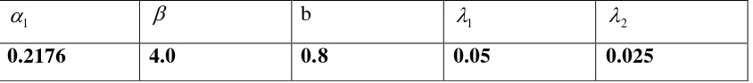
Table 8-1: Estimated parameters for beta distribution ... 156

Table 8-2: Variances and covariance for the estimated parameters ... 157

Table 8-4: Null hypothesis for Pearson product-moment correlation coefficient ... 162 Table 8-5: Conditional failure probability from a beta wear model and the residual time

NOTATIONS

k j

i, , Integers counter

t Monitoring Time

i

X ,Y_i Random variable at time t_i

i

x A realization of X_i, which is an underlying state of the equipment.

1. Defined as a residual time for a continuous case

2. Defined as true states for a discrete case, use Xi as the

notation.

i

y A realization of Y_i, the measurement obtained at time t_i by condition monitoring tools.

i

 The condition monitoring history obtained up to time t_i where _i 



y₁,y₂,y_i



) | (x_{i i}

P  Conditional probability of the underlying state (discrete case), given the history of condition monitoring. )

| (x_{i i}

p  Conditional probability density function of the underlying state (continuous case), given the history of condition monitoring (reflective variable).

) , | (x_{i i i}

p   Conditional probability density function of the underlying state (continuous case), given the history of condition monitoring (reflective and responsive variables).

i

 The condition monitoring history (covariates) obtained up to time ti where i 



z1,z2,zi



) | (xi xi_1

P Transitional matrix for a Markov chain

i

L Random variable for stage i duration with l_i is their realization.

) (

P Probability mass function

) (

p Probability density function

) (t

h Hazard function

) (

0 t

h Baseline hazard function

)) ( , (t z t

h Hazard function in the presence of a covariate z(t) )

(t

z Vector of covariates at time t

) (t

n Intensity function

) (

0 t

n Baseline Intensity function

) (t

Z Cumulative intensity function

Greek letters



, , , , , ,

, ₁ ₂ ₁  

 Parameters coefficient form chosen distribution ( e.g. Weibull and exponent) or parameters coefficient in a model.

p

C Cost of preventive replacement

f

Acknowledgments

I would like to express my gratitude to all those who have made it possible for me to complete this thesis.

My foremost thanks go to my supervisor Professor Wenbin Wang, for the patience and encouragement that carried me through difficult times, and for the detailed and constructive comments that helped to shape my research skills. Without him, this thesis would not have been possible.

I am deeply indebted to the late Professor A.H. Christer whose stimulating suggestions and encouragement helped me throughout this research.

I warmly thank other members from Centre for Operational Research and Applied

Statistics (CORAS), Dr. D.F Percy, Prof. H. Kobbacy, Dr. P. Scarf, Dr. D. Jackson, Prof. R. Baker, Dr. I. Mchale and Ms. S. Sharples, for their kind supports and guidances, which have been wonderful in this study.

During this work I was able to exchange ideas with many colleagues for whom I have great regard, and I wish to extend my warmest thanks to all those who helped me with my work.

I owe my loving thanks to my wife Rozilah Kamarudin, my daughters Nurul Syafiqah and Nurul Nabihah and my son Imran Tahir. Without their encouragements and understanding it would have been impossible for me to finish this work. My special gratitude is due to my family for their devoted and loving support.

Abstract

Condition monitoring and fault diagnosis for operational equipment are developing and showing their potential for enhancing the effectiveness and efficiency of maintenance management, including maintenance decision-making. In this thesis, our aim is to model the condition of equipment items subject to condition-monitoring in order to provide a quantitative measure to aid maintenance decision-making. A key ingredient towards dealing with the modelling work is to define the state or condition of the equipment with an appropriate measure and the observed condition monitoring may be a function of the state or condition of the operational equipment concerned. This leads to the two elements that are important in our modelling development; the need to develop a model that describes the system condition subject to its monitoring data and a decision model that is based upon the predicted system condition.

A quantification of the system condition in this thesis is modelled using either discrete or continuous measures. In the case of a discrete state space, this thesis presents details of how the initiation of a random defect can be identified. In the case of a continuous state space, two approaches, which were used to identify the system condition, are

1

CHAPTER 1: INTRODUCTION

1.1

Background and Motivation

Operational equipment such as pumps, conveyors, motors and others generate a large number of signals that can be monitored. As the parts of the equipment move and rotate, they produce vibration, sound and may change temperatures and pressures. In addition, the condition of the oil used as a lubricant also has a significant effect on the working condition of the equipment. These signals can act as maintenance indicators, which could be used to describe the key relationship between equipment condition and a maintenance decision. Using these condition-monitoring signals, we could assess equipment condition in its present operating environment and maintenance actions are

carried out only when necessary. This could result in a safe, effective and economical maintenance operation. Furthermore, the importance of condition monitoring in maintenance has been increasingly recognized, due to the availability of modern condition monitoring technologies. With these technologies, continuous conditional indicators are provided, which can help maintenance departments to develop, measure and improve maintenance actions in the organization.

However, most of these developments focused on the technical aspects of condition monitoring (Rao, 1995; 2001; 2002; 2003), such as advanced tools and techniques in monitoring technologies, signal processing, data acquisition and interpretation. These are mainly for diagnosis on issues of what to do, but the issue of when to do it received less attention. Yet, deciding when to do it (preventive repair) also requires some justifications.

It is a common practice that a certain threshold value has to be set for a chosen condition monitoring parameter of the equipment. The threshold level may be set up

based upon manufacture recommendations, personal experiences or other subjective criteria to provide a warning that a significant change has occurred and immediate action needs to be taken. From the condition-based maintenance perspective, this threshold level may not be optimal. This is due to the fact that each machine is an

so such a common threshold level is not appropriate in most cases. Furthermore, setting up a common threshold level may pose a difficulty for maintenance actions, and would incur extra costs. For example, if we set up a lower threshold value, it may result in needing more early replacements, and could waste much of the useful remaining lifetime of the equipment. In contrast, if we set up a higher threshold value, it will result in an increase of machine failures.

Thus, from an economical or safety point of view, the basic idea is to use all the monitored data (current and past) of a particular system, and make corresponding decisions to maintain the production equipment based upon cost, safety or other criteria. There is obviously a need for an appropriate model to aid such a decision support for

plant maintenance managers. It is noted however, only a very few tools are available in the market and only a small amount of research has been devoted to this area. Thus, developing a suitable model for effective decision-making in condition-based maintenance is regarded as an important addition to the subject.

To achieve our primary goal as described above, this research aims to predict the underlying state of a piece of production equipment, given its observed condition monitoring measurements at each monitoring point to date. How to define the underlying state of the equipment is a difficult issue and in this thesis, we used residual time and wear as examples. The residual time is chosen due to the fact that it represents an important characteristic in deciding an appropriate maintenance decision such as when to replace the equipment (Reinertsen, 1996). Similarly, cumulative wear could also be used, as it is a direct indication of the deterioration process. If these underlying states can be predicted, maintenance actions including manpower, equipment and tools, and spare parts can be planned and scheduled (Al-Sultan and Duffuaa, 1995).

In this study, by using available monitored-condition information, we believe that prediction of the underlying state could be much better than the conventional method, which uses only the current age to predict the remaining life or wear of a machine. It is noted that the result of the underlying state prediction can only be described by a

distribution is a key element in the subsequent maintenance decision model that we aimed to achieve.

However, there are several critical challenges, which make the establishment of the underlying state distribution a difficult problem. The first challenge is how we can define the failure, based upon the chosen underlying state and its relation to the observed monitoring data. That is, how well the condition monitoring data reflects the deterioration or failure process. Hence, understanding and modelling the processes of deterioration and failures themselves become essential in this research.

The second challenge is that we may have rich sources of condition-monitoring data but

very little failure information. Also as reported by Ascher et al. (1995) the data captured from the field suffers from many problems and it makes the data manipulation task both important and challenging. Hence, most of the effort has been placed on understanding, manipulating and preparing the data for development of the model.

The third challenge is that we may have a good theoretical model, but can it be implemented in real applications? Scarf (1997) surveyed the available papers on modelling condition-based maintenance and appealed for the applicability of the models in practice. Applicability in this case implies how the complexity and computation time can be reduced. Therefore, in developing the model, a few assumptions have been made, not only to simplify our modelling but also to ensure practical advantages.

To overcome all the challenges stated above, the objectives of this research are as follows:

1. To investigate the appropriateness of the defined state used in the model to quantify

the equipment condition.

2. To identify ways in which established model can be improved. 3. To explore approximation solution for the analytical model.

The following section contains an outline of the thesis, and gives an overview of the work.

1.2

Organization of the Thesis

This thesis is organized in nine chapters. In Chapter 1, we first introduce the common problems arising in condition-based maintenance and their challenges, which motivate us to carry out this research.

In Chapter 2, a brief introduction to maintenance and management strategy in undertaking maintenance actions is presented. We introduce the concept of condition monitoring and condition-based maintenance in detail. We investigate the literature and current monitoring techniques used within industry. It is noted that the scope of the literature review is mainly concerned with the modelling aspect of decision making in condition-based maintenance, thus several approaches and concepts related to this issue are discussed.

Chapter 3 presents a new development of a conditional residual time model that is different from the literature as reviewed in Chapter 2. A discrete state space is used to define the condition of the operational equipment. The methodology and formulation used in this development are discussed, and simulation studies with numerical results are presented. In this chapter, we show how the development of this model can be used to predict the initial point of a random fault in a system. The process of model fitting and testing using an actual dataset is shown in Chapter 4. Also in Chapter 4, we had an attempt to compare our results with a statistical process control based method, which had been developed in a previous study conducted by Zhang (2004).

In Chapter 5, we investigate numerical approaches as an alternative solution to the model developed in Chapter 3. Approximate approaches, such as grid based and particle filtering, are discussed. We demonstrate these approaches using simulated and actual datasets from Chapter 4.

values and many unexplained, so we have to re-organise the data into a format that is suitable for our model. One of the processes of re-organising the data is by transforming the collected data into a measure known as the total metal concentration. In general, three components of data are available to us such as the metal elements, lubricant performances and contaminant indicator while conducting the oil analysis programme. In this chapter, we only used the metal elements component indicator as it provides important information about the wear of the internal engine parts. Although there are many metal concentrations in the oil sample, not all of them are useful. Hence, a technique to reduce the dimension or size of metal elements is discussed. In addition, several procedures dealing with incomplete data are also presented. The model developed is fitted to the data and the numerical results are given. We carried out

several tests to show the robustness of the model developed, and produced significant results.

In Chapter 7, the model developed in Chapter 6 is enhanced with more monitoring

information. Using all three components presented in the oil-monitoring data, we grouped them into two groups. Here, we consider that these two types of condition-monitoring information are not correlated with each other but have different relationships with the residual life. The assumption and formulation for the new model are discussed, with a focus on interpreting and preparing the data required in the new model. As the lubricant performance and contaminant indicators are significantly correlated, we carry out an independent component analysis to separate each variable. The model is supplied with the actual data and the numerical results are given. Several other tests are also conducted.

As seen from Chapters 3, 4, 6, and 7, the residual time is used to characterize the failure or deterioration process of the production equipment. But, in Chapter 8, we attempt to model the deterioration process using a measure called ―wear‖, without using the residual time concept. To do this, we introduce a model that uses a continuous random variable to represent the process of deterioration of the system at any monitoring point. This is done using a beta distribution and allows us to have a more generic wear model

2

CHAPTER 2: LITERATURE REVIEWS

2.1

Introduction

This review of literature is divided into three sections, according to the nature of the problems discussed. The first section introduces the area of maintenance in general, the second section covers the concept of condition-based maintenance and its components, and the last section is concerned with the modelling aspects of condition-based maintenance, designed to aid maintenance decision-making. A fundamental understanding of the above topics is essential to the conduct of this research.

2.2

An Introduction to Maintenance

The purpose of system maintenance is to ensure the viability of the operation of equipment, as most equipment will deteriorate while in operation and with the lapse of time. A consequence of the deterioration process may be a failure of the system. Some failures are minor and result in inconvenience and small economic loss, while other failures are catastrophic, lead to uncountable cost and may be dangerous to personnel. There are many contributory factors to deterioration such as degradation, corrosion, wear, erosion, aging and production process are known as some of the root causes; and maintenance is necessary to prevent equipment from continuously deteriorating and suffering breakdowns (Reinertsen, 1996). Therefore, a well-planned maintenance

scheme is important in reducing costly breakdowns (Dohi et al., 2001) while at the same time maintaining a high level of quality (Paz and Leigh, 1994) or improving the viability of the system (Murthy and Hwang, 1996).

Formally, maintenance has been defined by BS EN 13306:2001 as

Combination of all technical, administrative, and managerial actions during the life cycle of an item intended to retain it in, or restore it to, a state in which it can perform the required function.

A more general understanding of maintenance is given by Pintelon and Gelders (1992) as

all activities necessary to restore equipment to or keep it in a specified operating condition.

This would imply that maintenance consists of actions taken to make sure that items of equipment are fit to fulfil their required functions. It should be noted here that we should have a clear notion of the meaning of ‗required function‘ or ‗specified operating condition‘ as stated in the above definitions. It should be understood that equipment is usually designed with some pre-defined life expectancy or operational life. For example, equipment may be designed to operate at a full design load for such amount of age or usage. In the case of an engine, belts and hoses need adjustment, alignment must be maintained, and proper lubrication on rotating equipment is required. Such a specification of the design life assumes necessary maintenance and any failure to perform maintenance activities intended by the equipment‘s designer would shorten its operating life.

Performing maintenance activities requires justification, as it contributes to cost, safety

and other criteria. Jabar (2003) divides maintenance costs into two main groups namely direct and hidden costs. The former consist of items such as labour, materials, services and overheads, while hidden or indirect costs are harder to measure and are classified into six main areas of losses:

1. Breakdowns and unplanned plant shutdown losses. 2. Excessive set-up, changeovers and adjustments losses. 3. Idling and minor stoppages.

5. Start-up losses. 6. Quality defects.

An attempt should be made to ascertain how maintenance can be performed to ensure equipment reaches or exceeds its design life, taking into account economic considerations, safety or other criteria. Therefore, it is very important for companies to have a good maintenance strategy for managing the effectiveness of maintenance and maximizing equipment uptime in their organizations. A review of the maintenance objectives is summarized by Wang et al. (2004) as follows:

1. Ensuring system function (availability, efficiency and product quality). 2. Ensuring system life (asset management) and safety.

3. Ensuring human well-being.

To accomplish the maintenance objectives above, three types of maintenance policies

have been used such as corrective, preventive and condition-based maintenance. Corrective or breakdown maintenance has been used for many decades and is still in practice today (Luce, 1999). The basic principle of, ‗fix it when it fails‘ is an approach where no preventive maintenance activities are carried out until failure occurs, when maintenance is resorted to in order to restore the required function. As a result,

1. Equipment or machines may be exposed to catastrophic failure. 2. Excessive secondary damage may occur.

3. Production downtime during excessive maintenance repair time is very costly.

4. Parts are not always readily accessible and may be expensive. 5. There is danger to the operating personnel and environment.

To minimize the impact of unexpected equipment breakdown or failure, maintenance practitioners started to adopt what was known as a planned preventive or time-based maintenance policy (Silver and Fiechter, 1992). This strategy aims at preventing

simple to manage. However, the difficulty in determining the appropriate time to perform maintenance and the need to interrupt production at scheduled time points reduce the impact on saving maintenance costs, as claimed by Swanson (2001).

The requirement for increased plant productivity associated with plant automation and the need for improved safety and reduction in maintenance costs have led to the growth in popularity of condition-based maintenance (CBM), which uses various condition monitoring techniques to aid the planning of plant preventive maintenance and operational policies (Christer et al., 1997). With condition monitoring, the signals of system deterioration may be easy to observe, hence equipment maintenance can be scheduled at the appropriate time and not on an emergency basis. Therefore, the plant availability can be increased and the cost of unscheduled production shutdowns can be

reduced.

In practice, however, the choice of the optimum maintenance strategy is not as simple as suggested above, as industry has become aware of the fact that a single maintenance

policy, however efficient it may be, cannot eliminate all breakdowns or restore the plant to its full potential (Saranga, 2002). Nowlan and Heap (1978) coined the term Reliability Centered Maintenance (RCM) in 1978 while writing a report on aircraft maintenance policy for United Airlines. Since then, the term was popularly adapted to be used in other maintenance industrial application. Formal definition of RCM is given by Moubray (1997), which stated RCM as

a process used to determine the maintenance requirements of any physical asset in it operating context.

In short, RCM is a structured procedure for analyzing the functions and potential failures of physical assets in order to determine and apply the most appropriate

This research is limited to investigating CBM as an option in maintenance decision-making, as it shows dominance over other two strategies. Kimura (1997) offers four reasons in support of this argument:

1. When the reliability of the item does not follow the ‗bathtub‘ curve, time

-based maintenance loses its significance.

2. If preventive maintenance is perfectly performed, resulting in no failure, then

we cannot have failure statistics.

3. Time-based maintenance is inapplicable to a new item for which failure statistics do not exist.

4. The development of a condition-monitoring tool and techniques has facilitated the implementation of CBM.

Hence, the next section will further discuss the CBM strategy and its components.

2.3

Condition-Based Maintenance

The purpose of CBM is to allow maintenance to be done only when necessary, with the help of condition monitoring data. As Kelly and Harris (1978) stated, the only aspect of CBM that distinguishes it from both run-to-failure and timed-based preventive

maintenance is the sense that it requires the monitoring of some condition indicating parameters of the unit being maintained. Run-to-failure maintenance requires no monitoring activities, while time-based preventive maintenance is based on statistical failure data and some sort of simple manual inspection. Referring to BS EN 13306:2001

CBM is defined as

Preventive maintenance based on performance and/or parameter monitoring and the subsequent actions.

actions can be carried out to prevent the equipment from failing completely or causing more damage to the plant. This statement illustrates the scope of condition monitoring as the techniques that can be used to identify warning signs by measuring any significant deterioration indicated by changes in the values of monitored variables. Moubray (1997) introduced the concept of P-F (Potential failure-Functional failure) curves; these are intended to explain his statement, as shown in Figure 2-1 below.

Figure 2-1: P-F curve

P refers to the earliest time at which a potential failure can be detected and F refers to the time at which the functional failure occurs. If a potential failure or fault can be detected between points P and F or earlier, a possible maintenance action can be

performed to prevent the functional failure from occurring. Moubray (1997) also mentions that there are many ways of finding out that failure is in the process of occurring. As an example, consider the P-F curve in Figure 2-2 below, which illustrates how the single failure mode could be preceded by a variety of potential failures, each of which could be detected by a different condition-monitoring technique defined by P1, P2,

Figure 2-2: Detection of potential failures

An alternative way to understand condition monitoring is to look at the delay time concept, introduced twenty years ago by Christer and Waller (1984), which is a model for industrial inspection maintenance problems. The concept has a similar definition to the P-F interval, but allows far more insight into the failure process. It defines failure as a two-stage stochastic process, where the first stage is the initiating phase of a defect, which was not defined in Moubray (1997). The second stage is where the defect leads to a failure in the absence of maintenance actions. The time lapse from the time a defect can be first identified at an inspection point, u, to the time that the defect causes a

failure, is called the delay time, h. If an inspection is carried out during this (variable) time period, the defect may be identified and removed. Figure 2-3 below illustrates the delay time concept.

Figure 2-3: Delay time concept

These concepts are sufficient to provide a practical view of condition monitoring and its consequences. Formally, BS EN 13306:2001 defines condition monitoring as

Note that, if the measured condition parameters have not changed, it does not mean that the monitoring is a waste of time. It provides a peace of mind that the equipment may be in a satisfactory condition. Also, if the measured parameters did not show any trend or change until failure, it is likely that a wrong type of information was collected. Thus, the brief discussion of condition monitoring above enables us to interpret condition-based maintenance as an outcome of the measurement of the system condition, condition-based on information called condition data with the aim of determining required maintenance actions. Therefore, CBM is shown to be a method which attempts to provide a diagnosis and prognosis approach towards maintenance problems. These analyses describe the processes of the assessment of equipment health for present and future, based upon

observed data and available knowledge of the system (Mathur et al., 2001).

Here, diagnosis is concerned with identifying the causes of failures or anomalous conditions in a system or its subsystems and determining the severity of given faults

once detected. Prognosis, on the other hand, is a very challenging task, which aims at predicting failures, based on observed data and available knowledge of the system, and may lead to recommending preventive maintenance prior to the onset of catastrophic failures.

2.4

Components of Condition-Based Maintenance

Wang (2000) while reporting a review of the modelling of CBM decision support

claims that there are two stages of condition-based maintenance. The first relates to condition-monitoring data acquisition and its interpretation, followed by the second stage of making a decision based on the monitored information. Similar arguments also can be found in Jardine et al. (2005) suggesting that a CBM programme should consist of three key steps:

1. Data acquisition, to obtain data relevant to system health.

2. Signal processing, to handle the data or signals collected in step 1 for better

understanding and interpretation of the data.

Hence, we may conclude that the theory and implementation of condition-based maintenance must have these components. The first component, data acquisition, plays an important role in this approach, in which the condition of the equipment needs to be known. In general, condition monitoring can be divided into two categories (Kelly and Harris, 1978), namely monitoring which can be carried out without interruption of production, and monitoring which requires the shutdown of the unit. This categorization is important in order to select the appropriate techniques and tools for data acquisition (Shearman, 2001). Attempting to fulfil this requirement, various data acquisition techniques and tools can be utilized within condition monitoring (Williams et al., 1995). Vingerhoeds et al. (1995) discussed additional kinds of condition monitoring, i.e.

off-line condition monitoring and on-off-line condition monitoring. The diagnostic system for on-line monitoring enables quick and reliable fault diagnosis for the warning that occurs. However, many challenges still exist in practical applications of on-line monitoring, such as rapid data processing, diagnosis procedure and the high operating

cost. To overcome such problems, off-line monitoring approaches have been used, in which the data is measured on-line but the analysis is carried out on a regular basis (off-line).

However, a key difficulty in condition monitoring is to detect changes that are not necessarily directly observed and that are indirectly measured together with other types of noise. In a study of the condition monitoring of a component which has an observable measure of condition called ‗wear‘, Christer and Wang (1995) classify the information collected during the monitoring exercise into two categories, namely direct and indirect information. They define the direct information as the measurement of a variable that can directly determine the state of the system, for example the thickness of a brake pad or the depth of a crack. Normally, these direct methods may be based on

visual inspections or other types of monitoring such as non-destructive sensing which may not be economical to use for some equipment (Jantunen, 2006). Indirect information is defined as the associated information that is influenced by the component condition, which cannot be directly observed; for example, the information gathered in

Another categorization is found in the work of Martin (1994) who distinguishes between two different types of fault, namely soft and hard faults (see Figure 2-4). The difference between these types is important, as soft faults lead to predictable situations, hence being amenable to condition monitoring, while hard faults are basically unpredictable; but there is a view that even hard faults must exhibit some changes before the occurrence of the failure (Martin, 1994).

Figure 2-4: Hard and soft failures

One example of such a categorization is that a large amount of recent industrial research has put more effort into systems consisting of mechanical plant and equipment such as power turbines, diesel engines and other rotating machinery, rather than electronic or electrical systems. The reason for this is that failure in mechanical systems tends to occur slowly, so that if condition monitoring is performed, it will provide an

opportunity to assess the deterioration and to compute the expected remaining life of a system or machine, while in electronic systems, failures tend to occur without any warning or delay time.

Others (Andersen and Rasmussen, 1999) have referred to it as ‗information about technical health‘. It has been reported that major improvements have occurred in the technology, practice and use of equipment condition monitoring over the past sixty years (Mitchell, 1999). An example is the development from the mechanical instruments that were used 20 years ago to capture a simple low frequency dynamic waveform to today‘s high-performance digital instrumentation. Methods of equipment condition monitoring can be classified according to the monitored parameters that were influenced by the potential failure (Moubray, 1997). To support his argument, Moubray divides condition-monitoring techniques into six categories:

1. Dynamic effects, such as vibration and noise levels. 2. Particles released into the environment.

3. Chemicals released into the environment.

4. Physical effects, such as cracks, fractures, wear and deformation. 5. Temperature rise in the equipment.

6. Electrical effects, such as resistance, conductivity, dielectric strength, etc.

However, irrespective of the condition monitoring techniques used, the key elements of condition monitoring are the same: the condition data that becomes available needs to be converted into a meaningful form and appropriate actions must be taken accordingly. As examples in this discussion, a few condition monitoring techniques that are popular in industry have been selected from the survey conducted by Higgs et al. (2004). For other references to such methods, see (Moubray, 1997) and (Williams et al., 1995).

2.5

Condition-monitoring techniques

2.5.1 Vibration Monitoring

The changes at this stage may signal a warning of the impending failures that may occur. Reeves (1998) explains that vibration monitoring consists of identifying two quantities: the magnitude of the vibrations and their frequency. The former is used to establish the severity of the vibration, while the latter indicates the origin of the defect. It should also be noted that the severity of the vibration in any particular case would depend on these factors:

1. Type of machine

2. Flexibility of the mounting/foundation 3. Position or direction of measurement 4. Operating conditions during measurement

A summary of techniques used in vibration monitoring is given by Reeves (1998).

2.5.2 Oil Analysis

Condition monitoring through oil analysis provides a means of analysing oil at regular intervals to determine if it still meets the lubrication requirements of the equipment. The

particles contained in a lubricating fluid carry detailed and important information about the condition of the machine components. There are many methods, which can be utilised to perform an analysis to obtain such information. A comparison between different methods, which were available, is given by Roylance (2005). The features of the analysis can be deduced from particle shape, size, composition, size distribution and concentration, which can be classified into three categories namely quantitative, qualitative and material properties, see Khan and Starr (2006) for details of the classifications.

A change in the rate of particles collected indicates a change in the condition of the machine. When this condition reaches an unacceptable state, the machine must be replaced to maintain satisfactory system operations. The two most commonly used

this method monitors only the smaller particles present in the oil (<10 microns). This disadvantage of spectrometric analysis is due to the fact that large and medium particles (> 10 microns) are likely to exit the oil flow via some filtration. This leaves the small particles which passed through the filter to remain suspended within the engine and their oil measurements to provide an indication of machine condition (Edwards et al., 1998).

Ferrographic analysis produces similar results to spectrometric analysis, but with two main exceptions. First, ferrographic analysis separates wear particles by using a magnetic field, rather than burning a sample as in spectrographic analysis. Secondly, wear particles that are larger than 10 microns can be separated and analysed, which

provides a better representation of the wear particles in used oil analysis. The only criticism of this technique is that the analysis of the wear particles is very skill-dependent, subjective and time-consuming as well (Whitlock, 1997) and (Roylance, 2005).

2.5.3 Temperature Monitoring

Thermography has become a common technique for non-destructive inspections in various engineering fields which is mention by Lo and Choi (2004). It allows the monitoring of temperatures and thermal patterns to be conducted while the equipment is in operation. Generally, all mechanical systems generate thermal energy during normal operation, which permits infrared thermograph instruments such as infrared detectors to evaluate their operating conditions. Thermal anomalies, where components are colder or hotter than they should be, are taken as alarm signals of potential problems within the system. However, Lo and Choi (2004) conclude that these results can also be affected by the experience of the assessor, equipment capabilities, construction details and environmental factors.

2.6

Data Interpretation

processing. The purposes of signal processing in diagnostic and prognostic applications of CBM are given by Bengtsson et al. (2004) as:

1. To remove distortions and restore the signal to its original shape.

2. To remove sensor data that is not relevant for diagnostics or predictions. 3. To transform the signal to make more explicit any relevant features, which

may be hidden in the signal.

This also correlates with the work of Mathur et al. (2001) who noted that the real issues in signal processing are features of selection/reduction and how to treat any missing data. In addition, they noted that two characteristics that are common to all applications

are incomplete or imprecise knowledge about the system of interest, especially in the failure space, and the uncertainty of the observed data. In certain cases, signal processing may also manipulate the signal so that some characteristics become more visible, enabling better prognosis. An example of the data cleaning procedure is

introduced by Jardine et al. (2001) in monitoring the condition of mine haul truck wheel motors. Another example is given by Christer and Wang (1992), who assumed that condition monitoring is capable of indicating wear trends, which can then be used to determine the critical warning level and frequency of monitoring inspections.

2.7

CBM Decision Making

(Prabhakaran and Jagga, 1999) and implementation of computerized condition monitoring (O'Sullivan, 1991; Bekiaris and Amditis, 2003). Recent developments in artificial intelligence such as neural networks (Timusk and Mechefske, 2001), expert systems, fuzzy logic (Liu et al., 1996) and genetic algorithms also contribute to the techniques of fault diagnosis.

The third problem mentioned above (Tsang, 1995) relates to decisions on how and when to schedule the condition inspections in an effective way. Decision-making in this perspective is concerned with the selection of an economic inspection schedule to balance the cost and downtime due to breakdowns and inspections. Grall et al. (2002) reporting on the CBM policy for a stochastic deterioration system, state that the choices

made in determining the monitoring intervals and establishing the critical threshold values will influence the economic performance of the maintenance policy, so that, in practice, a conservative approach could lead to the setting of a threshold and inspections being conducted more often than necessary, leading to non-optimal maintenance

policies. As an example, Wang (2000) presented a model dealing with the selection of the best condition monitoring interval and the optimal critical level in terms of a criterion of interest, which can be cost, downtime or reliability.

Now, let us consider the action to be taken at the time of each inspection or monitoring; at this point, two decisions will be made: first, what maintenance action to take, either to replace or repair the system to a specific state or to leave as it is; and secondly, when the next inspection will take place (Lin and Wiseman, 2005). Again, the decision at this stage can be complicated and entails considerations of cost, downtime, production demand, preventive maintenance shutdown windows and most importantly, the likely survival time of the item monitored. Implementation of condition monitoring costs money, and therefore the purpose of condition-monitoring strategy development is to

ensure the optimum return by maximizing the effectiveness of the monitoring data.

Jardine et al. (2005) state that most companies are very enthusiastic in their general commitment to CBM, but often confined themselves to the data acquisition step,

remaining life. Hence, an unknown amount of remaining life is wasted and this does not afford the end-user any means of economically evaluating condition-monitoring data. A good example of this is a study of the oil-based condition monitoring of locomotive gearboxes used by the Canadian Pacific Railway (Aghjagan, 1989), which indicated that the failure rate of gearboxes while in use fell by 90% after condition monitoring was commissioned; however, further details of reconditioning/overhaul showed that there was nothing evidently wrong in 50% of the cases. Obviously, this is not an efficient way to perform CBM. An effective and efficient CBM programme must include not only advanced condition-monitoring equipment for data acquisition but also advanced technologies for signal processing and maintenance decision making.

This can lead to a challenge regarding how to build up an appropriate formulation for learning and inference concerning problems of maintenance decision making using condition-monitoring data. Lofsten (2000) defines maintenance modelling as a mathematical model used to represent the behaviour of the plant under different maintenance actions and thereby to identify the ‗best‘ maintenance decisions in terms of cost, downtime, output, availability or any criterion of interest. Further details of model development are discussed by Dekker (1995), according to whom maintenance optimisation models should address four aspects:

1. Description of a technical system, its function and its important features. 2. Modelling of the deterioration of the system over time, and possible

consequences for the system.

3. Description of the available information about the system and the actions open to management.

4. An objective function and an optimisation technique, which help in finding

the best balance.

However, because at the early stages decision making was not emphasized, or justified via quantitative rather than qualitative measurement, little attention has been paid to modelling the appropriate decision making in CBM (Wang, 2000). A related argument

literature shows that modelling CBM is under-explored and the few related studies available are small in number, having been conducted by the same groups of authors.

Only a few of the papers, which have been assessed, are based on the types of monitoring data. Christer and Wang (1995) developed a simple monitoring model based on direct condition information. Hontelez et al. (1996) developed an optimum CBM policy for deteriorating systems based on a Markov decision process. Aven (1996) developed a condition-based replacement policy using a counting process approach. A model based on indirect monitoring information has been presented by Wang et al. (1997) and Christer et al. (1997). Wang and Christer (2000) used the filtering approach in modelling the residual time distribution subject to condition monitoring. Love and

Guo (1991), Kumar (1996) and Jardine et al. (1998) used a ‗proportional hazards‘ model as an attempt at modelling CBM.

A study by Wang et al. (1996) on stochastic decision modelling of CBM shows how a

relationships between the condition of the system and monitored information can be established. Wang et al. (1996) using a regression model to predict the future condition information and an accelerated life model to predict the future development of the true condition of the system. Based upon the accelerated life model, a decision model can be established to determine the decision variable of interest, such as the optimal replacement time. Later, a study done by the same author Wang (2000) used a random coefficient growth model to describe the deterioration process of an item monitored to explore the relationship between the critical level, monitoring intervals and the objective function of interest. Scarf (1997) surveys the available papers on modelling CBM and appeals for the applicability of the models in practice. He finds that too much attention was being paid to the invention of new models without practical implementation. In particular, this criticism recognizes that since CBM is based on monitored data, the

2.8

Modelling in Condition-Based Maintenance

The objective in developing a CBM model is to acquire knowledge about the equipment condition based upon its monitored parameters, so that any necessary maintenance decisions can be made accordingly. Generally, models can be divided into two parts: the deterioration model and a decision model (Frangopol et al., 2004). The deterioration

model is used to approximate and predict the actual deterioration process, taking into consideration age and condition-monitoring information. The decision model uses the deterioration model to determine the optimal decision that we would like to decide in order to minimise a criterion of interest, such as cost, safety and others. Since the current and future states of a system are unknown unless it is directly observed, a probabilistic approach is suitable for the model.

In this section, a general idea is given on how this uncertainty is modelled as a key element of CBM optimisation. Several approaches are being researched and applied in the development of CBM models. One of the methods that have been widely used is Proportional Hazards Modelling (PHM).

2.8.1 Proportional Hazards Model (PHM)

Introduced by Cox (1972), the Proportional Hazards (PH) model is used to identify significant covariates and to quantify their effects on survival (using hazard function) as a function of covariate values and the working age (time). The model has been widely used in the biomedical field, for which medical research and drug trials are examples.

[image:37.595.134.503.74.280.2]

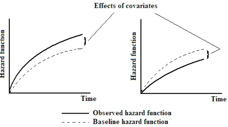
Figure 2-5: Illustration of pattern of the hazard function and the baseline hazard function.

Kumar (1996) stated that effect of a covariate is to increase or to decrease the hazard function. Mathematically, the hazard function can be written as

)) ( , ( ) ( )) ( ,

(t z t h₀ t z t

h    (2-1)

where h₀(t) is the baseline hazard function, (,z(t)) is the functional covariate term, )

(t

z is a vector of covariates and  is a vector of covariate coefficients. These

covariates may be measurements of machine condition, such as the levels of metallic

components in oil analysis or vibration amplitude.  may be estimated from the data to

provide a quantitative measure of the importance of each covariate and their impact on the hazard.

To use PHM, a stopping rule (the interval for maintenance) needs to be defined. In

Jardine et al. (1997) and Jardine et al. (1998), the interval is defined as T_d, where d 0. To find the optimum value of d, the cost model (Jardine et al., 1998; Kobbacy et al., 1997) is used, and shown below

) (

) ( ))

( 1 ( ) (

d W

d Q C d Q C

d

where

p

C is the mean cost of a preventive replacement.

f

C is the mean cost of a failure replacement. )

(d

Q is the probability that an item will fail before a preventive replacement.

) (d

W is the expected time between two consecutive replacements (regardless of reason

for replacement – preventive or at failure).

The details of this formulation can be found in Jardine et al. (1998). The two most common techniques for estimating the PHM coefficients are (i) Cox‘s partial likelihood method, which estimates the coefficients without making any assumptions about the form of the base hazard, and (ii) the maximum likelihood estimation (MLE) method, in which an explicit form of base hazard (e.g. Weibull hazard) is assumed (Gurvitz, 2005).

Higher values of  will reduce the estimated survival time for a machine, so it can be

viewed as a factor accelerating the failure rate of the machine (Mann et al., 1995).

Jardine et al. (1998) consider the baseline hazard h₀(t) as a Weibull hazard function, which has the following form

1

) (



      



 

 t

t

h_o (2-3)

where  and  are the scale and shape parameters. Once the optimal threshold level

*

d is calculated, it is easy to utilize the optimal replacement rule where the replacement is taking place at the first time t for which

t d

t z t

z₁( ) _{2 2}( ) ln * ( 1)ln

1    _   

 

   (2-4)

This implies that PHM combines all the significant measurements into one single value with appropriate weights. The decision rule then suggests preventive replacement at the time t when the combined covariate values reach the warning level, which depends on

condition monitoring process (Jardine et al., 2001; Love and Guo, 1991; Vlok et al., 2002). A list of applications of PHM in reliability studies can be found in Kumar (1996). The advantage of this method is that it includes both the age and the condition of the equipment in the calculation of the hazard at time t (Jardine et al., 1998). Needless to

say, PHM assumes that the covariates will change the hazards that may be true in some cases, but in reality it may be the state of the system that causes the change in the observed parameters and not vice versa, such as in the case of vibration monitoring. This would be a significant problem if PHM were used in CBM, where the relationship between the monitored parameters and the underlying state of the system does not follow the assumptions made in PHM.

2.8.2 Proportional Intensities Model (PIM)

Another approach used in modelling CBM is the proportional intensities model (PIM), in which the proneness of the unit to failure can be characterized by the failure intensity. A typical example of this type of problem is a repairable system, in which, when the failure occurs, a small part of the system can be repaired without replacing the entire system. The system may be repaired several times before being finally replaced; therefore a system that is considered repairable cannot be modelled by the conventional

hazard function, as successive failures are not identically distributed and not independent. Instead, it can be modelled using a counting process in which the hazard function with time-dependent covariates can be replaced with the intensity function, which may be defined in terms of the number of failures, N(t) over time (0,t). In other

words, this describes the failure intensity. Wang (2000) defines the intensity function with a baseline intensity multiplied by a multiplicative factor involving covariates, which can be written as

)) ( exp( ) ( )

(t n₀ t y t

n   (2-5)

where n₀(t) is the baseline intensity and y(t) is a vector of covariates. A non-homogeneous Poisson process (NHPP) forms the basis of this model. Common models

used to describe the baseline intensity of an NHPP include the power law model, 1

0( )



_ 

t t

having intensity function n(t), then N(t) is a Poisson random variable having mean

) (t

Z , where Z(t)is the cumulative intensity function.





t

du u n t Z

0

) ( )

( (2-6)

Consider that the system has an increasing intensity function, which tells us that failures will be likely to occur more frequently and at some time t it will become more economical to replace the system. To find the optimum value of t, (t*), we minimize the cost model,



( )



1 )] (

[ C C Z t

t t C

E  _p  _f (2-7)

where

p

C is the cost of replacing/preventive the system.

f

C is the cost of a failure.

Such applications can be found in Aven (1996), Ascher et al. (1995), Percy et al. (1998) and Watson et al. (2002). PIM is just an extension of PHM (Kumar, 1996), which also assumes that the covariates will influence the intensity, hence it experiences the same shortcomings as those of PHM discussed above.

2.8.3 Markov Models

Another approach that is widely used for modelling CBM uses Markov models. In all cases of condition monitoring, the condition of a technical unit is changing continuously.

Figure 2-6: Illustration of 3 states Markov model

A transition probability



P₁₂,P₂₁,...P₁₃



is defined as the probability that a component will move from one state to another, depending on the action taken. The Markov property assumes that the probability of deteriorating to another state does not depend

on the history of the process, which implies that the future lifetime of a component/system does not depend on how long it has already operated. Applications of this approach in CBM can be found in Coolen and Dekker (1995) and Hontelez et al. (1996). However, the ‗memoryless‘ property of this approach, which considers the

future condition as dependent