Lab Notes PH-315
Portland State University A. La Rosa
Transfer function and the Laplace transformation
__________________________________________________________
1. INTRODUCTION
2. THE LAPLACE TRANSFORMATION
L
3. TRANSFER FUNCTIONS4. ELECTRICAL SYSTEMS
Analysis of the three basic passive elements R, C and L Simple lag network (low pass filter)
1. INTRODUCTION
Transfer functions are used to calculate the response C(t) of a system to a given input signal R(t). Here t stands for the time variable.
Physical system Electronic circuit, mechanical system,
thermal system
r(t)
Input signal
c(t)
Output signal
Fig. 1 Given an input signal, we would like to know the system response C(t).
The dynamic behavior of a physical system are typically described by differential (and/or integral) equations:
For a given input signal R(t), these equations need to be solved in order to find C(t).
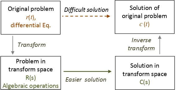
Alternatively, instead of trying to find the solution in the time domain, each time-variable, as well as the differential equations, can be transformed to a different variable domain in which the solutions can be obtain in a more straightforward way; then an inverse transform would take place the solution into the time domain
Difficult solution Original problem
r(t), differential Eq.
Solution of original problem
c (t)
Easier solution
Problem in transform space
R(s)
Algebraic operations
Solution in transform space
C(s)
Transform Inverse
transform
[image:1.612.168.451.535.680.2]One of those transforms is the Laplace transformation
2. THE LAPLACE TRANSFORMATION
L
The Laplace transform F=F(s) of a function f = f (t) is defined by,
f
LF
L
(f ) = Ff(t)
e
-stdt
0
F(s )
(1)
The variable s is a complex number, s = a +j.
t
f (t)
a
s
f
F F(s)
Time domain Laplace domain
Example f is the unit step function
t
f
dt
st -t f( )e
0
F(s )
=
1e
-stdt
0
=
s 1
(2)
Example A signal response from a system (temperature, for example) respond, after an e ter al; e itatio has stopped, de a i g e po e tiall . Let’s fi d out how su h de a is characterized by a Laplace transformation.
f is a decaying exponential f(t)A
e
-t
t
f
dt
st -t f( )e
0
F(s )
dt
st-e
e
- tA
0
F(s )
=
s A
(2)
Time domain Laplace domain
Example. As we mentioned in the introduction, the system response is governed by differential
equations. We would like to know then, how dt df
and 2
2
dt f d
transform by a Laplace
transformation. For simplicity, and clarity, let’s use the notation: dt df
= f ’ and 2
2
dt f d
= f ” . If F =
L
(f ) evaluateL
(f ’)L
s ) '
(f f'(t)
e
-stdt
0
f(t)
e
-
st f(t)e
-stdt
0
s
o
f(0) f(t)
e
-stdt
0
s
( ) [ (f )] s
s
L f 0
f(0)
sF(s) Laplace transformation of (3) the derivative
Typically, one proceeds putting the initial conditions equal to zero. (The situation with initial conditions different than zero are added in a separate simpler procedure). Thus,
L
s ) '
(f
s F(s) Laplace transformation of the derivative (3)’
with the initial conditions equal to zero
L
s ) "
(f f"(t)
e
-stdt
0
f'(0)
sf(0)
s2 F(s) Laplace transformation of the (4)
second derivative
Typically, one proceeds putting the initial conditions equal to zero. (The situation with initial conditions different than zero are added in a separate simpler procedure). Thus,
L
s ) "
(f
s2 F(s ) Laplace transformation of the second derivative (4)’
with the initial conditions equal to zero
Example. Sometimes the response signal of a system (the voltage across a capacitor, for example) must be given in terms of the integral of another quantity (the integral of the corresponding current across the capacitor). It is convenient, then, to obtain the Laplace
transformation of an indefinite integral g(t) t f(u)
du
0
If F =
L
(f ) and tdu
0 f u t
g( )
( ),
evaluateL
(g)
L
(g) s g(t)e
-stdt
0
t f u du
e
-st dt0 ( ) ]
[
0
t f u du
e
-st f te
-st dt0 s
1 [ ] ) ( [ s
1 ] ) ( [
-
]
0
0
f(t)
e
-stdt s1
0
F(s ) s 1
Laplace transformation of the (5)
indefinite integral
3. TRANSFER FUNCTIONS
Differential Eq governing the behavior
of the system r(t)
Input signal
c(t)
Output signal
Fig. 3 Schematic of the system response in the time domain
In a simple system, the output c(t) may be governed by a second order differential equation
Applying the Laplace transforms ’ a d ’, o e o tai s
( a2s2 + a1s + ao ) C(s) = R (s)
C(s) R(s ) a
s a + s a
1
o 1 2 2
In a more general case, the differential equation may be of higher order (higher than 2). Also the input may be composed of derivatives of a given function r=r(t). Therefore the factor
a s a + s a
1
o 1 2 2
may become a more elaborated function of s.
Thus, for a system in general,
C(s) = G(s) R(s) (6)
Notice, G=G(s) characterizes the physical system. It is called the transfer function.
It is more typical to write,
R(s) C(s)
G(s)
(7)
from which, for a given R=R(s) the function C=C(s) can be obtained.
G(s)
R(s)
Input signal
C(s)
Output signal
Fig. 4 Schematic of the system response in the Laplace domain
Example. A system is characterized by the transfer function 6) (s 1) (s
3 2s G(s)
.
Find out how the system respond to a exponentially decaying input r(t)
e
-2t .Answer:
The Laplace transformation of r gives, using expression (2), R(s) = 2 1
s
The output signal, in the Laplace domain , is then given by,
2 1 6) (s 1) (s
3 2s C(s)
s
2 s K 6 s K 1 s K
C(s )
1
2
3
, with K1, K2, K3, to be determined.Notice, K C(s )(s 1) 0.8 1
1
K2 C(s )(s6)6
-0.3
0.5 2) (s C(s )
K3 2
Thus, 2 s 0.5 -6 s 0.3 -1 s 0.8 C(s )
Now, using (2) we identify the time dependent functions these individual Laplace transforms come from,
c(t)
0.8
e
-t
0.3
e
-6t 0.5
e
-2t Answer.Recapitulating the process,
Difficult solution
Original problem
r(t)
Solution of original problem
c (t)
Problem in Laplace space
R(s)
Solution in Laplace space C(s) Laplace Transform Inverse transform t
-e
tr() 2
System Differential Eq
Integral Eq.
G(s)
+ algebraic operations
R(s) = 2 1 s 6) (s 1) (s 3 2s G(s) 2 s 0.5 -6 s 0.3 -1 s 0.8 C(s ) 2t -6t -t
-e
e
e
t 0.5 0.3 0.8 ) c( Fig. 5 Schematic representation of the solution procedure in the previous example.
4. ELECTRICAL SYSTEMS
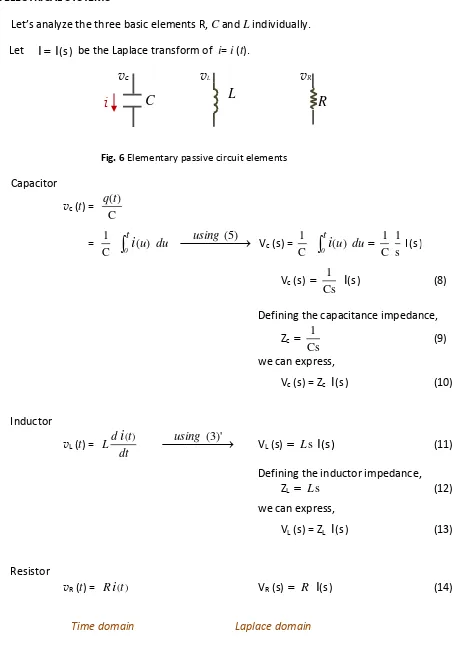
Let’s a al ze the three asi ele e ts R, C and L individually. Let
I
I
(s ) be the Laplace transform of i= i (t).
v
cL
C
R
i
v
Lv
RFig. 6 Elementary passive circuit elements
Capacitor
vc (t) = C
) (t q
= C 1
du u
t
0
i
( )
using(5)Vc (s) = C 1
du u
t
0
i
( )
I(s )s 1 C 1
Vc (s)
I
(s ) Cs1
(8)
Defining the capacitance impedance,
Zc Cs
1
(9)
we can express,
Vc (s) = Zc
I
(s )(10)
Inductor
vL (t) = dt
t d
L
i
( ) using(3)' VL (s) LsI
(s)(11) Defining the inductor impedance,
ZL Ls
(12)
we can express,
VL (s) = ZL
I
(s )(13)
Resistor
vR (t) = R
i
(t) VR (s) RI
(s)(14)
[image:7.612.84.544.84.734.2]
Analysis of a simple lag network
Solving the Kirchoff law in the time-domain and in the Laplace -domain
R
C
vout (t) vin (t)
q
i
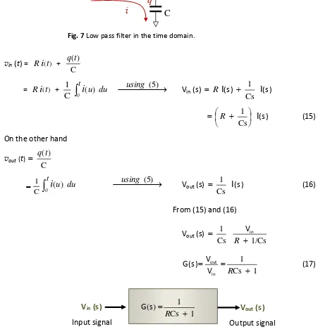
Fig. 7 Low pass filter in the time domain.
vin (t) = R
i
(t) + C) (t q
= R
i
(t) +C 1
du u
t
0
i
( )
using(5) Vin (s) RI
(s)I
(s ) Cs1
I
(s ) Cs1
R (15)
On the other hand
vout (t)
C ) ( q t
C 1
t u du
0
i
( )
using(5) Vout (s)I
(s ) Cs1
(16)
From (15) and (16)
Vout (s) Cs
1
1/Cs
R in V
1 Cs
1
R in out V V
G(s ) (17)
1 Cs
1 )
(
R
s G
Vin (s)
Input signal
Vout (s)
Output signal
Fig. 8 Low pass filter in the Laplace domain.
[image:8.612.89.540.148.623.2] Analysis of a simple lag network
Method using the complex impedance in the Laplace domain
R
ZC
Vout(s) Vin(s)
I(s)
Vin (s) = ( R ZC)
I
(s )
) Z
( C
R (s ) V
(s ) in
I
On the other hand,
(s ) (s )
Vout ZC
I
) Z ( Z
C C
R (s ) Vin
Using expression (9), Zc Cs
1
,
) Cs
1 ( Cs
1 ) (
R V s
V in
out ( )
1 Cs
1
s Vin
R
1 Cs
1 )
( ) (
R s V
s V G(s )