Improved Harmony Search Algorithm with Chaos for Absolute Value Equation

DOI: _{10.12928/TELKOMNIKA.v11i4.1384  835}

Improved Harmony Search Algorithm with Chaos for

Absolute Value Equation

Longquan Yong*1, Sanyang Liu2, Shouheng Tuo3, Kai Gao4

1,2,3,4

School of Science,Xidian University, Xi’an 710071, China

1

School of Mathematics and Computer Science, Shaanxi University of Technology Hanzhong 723001, China

*Corresponding author, e-mail: yonglongquan@126.com1, yonglongquan@gmail.com1, liusanyang@126.com2

Abstrak

Pada tulisan ini, pencarian harmoni plus chaos ditingkatkan (HSCH) disajikan untuk memecahkan persamaan nilai absolut (AVE) Ax - |x| = b, di mana A adalah matriks persegi sembaran dengan nilai singular melebihi satu. Hasil simulasi dalam memecahkan beberapa masalah AVE yang diberikan menunjukkan bahwa algoritma HSCH adalah valid dan lebih baik dari algoritma HS klasik (HS) dan algoritma HS dengan operator mutasi diferensial (HSDE).

Kata kunci: persamaan nilai mutlak, nilai singular, harmoni pencarian, kekacauan

Abstract

In this paper, an improved harmony search with chaos (HSCH) is presented for solving NP-hard absolute value equation (AVE) Ax - |x| = b, where A is an arbitrary square matrix whose singular values exceed one. The simulation results in solving some given AVE problems demonstrate that the HSCH algorithm is valid and outperforms the classical HS algorithm (HS) and HS algorithm with differential mutation operator (HSDE).

Keywords: absolute value equation, singular value, harmony search, chaos

1. Introduction

We consider the absolute value equation (AVE):

Ax



x



b

(1)

where

A



R

n n ,

x b

,



R

n _{, and}

x

_{denotes the vector with absolute values of each} component of

x

. A slightly more general form of the AVE (1) was introduced in John [1] and investigated in a more general context in Mangasarian [2].

As were shown in Cottle et al.[3] the general NP-hard linear complementarity problem (LCP) that subsumes many mathematical programming problems can be formulated as an absolute value equation such as (1). This implies that AVE (1) is NP-hard in general form. Theoretical analysis focuses on the theorem of alternatives, various equivalent reformulations, and the existence and nonexistence of solutions. John [1] provided a theorem of the alternatives for a more general form of AVE (1),

Ax



B x



b

, and enlightens the relation between the AVE (1) and the interval matrix. The AVE (1) is shown to be equivalent to the bilinear program, the generalized LCP, and the standard LCP if 1 is not an eigenvalue of

A

by Mangasarian [4]. Based on the LCP reformulation, sufficient conditions for the existence and nonexistence of solutions are given.

It is worth mentioning that any LCP can be reduced to the AVE (1), which owns a very special and simple structure. Hence how to solve the AVE (1) directly attracts much attention. Based on a new reformulation of the AVE (1) as the minimization of a parameter-free piecewise linear concave minimization problem on a polyhedral set, Mangasarian proposed a finite computational algorithm that is solved by a finite succession of linear programs [7]. In the recent interesting paper of Mangasarian, a semismooth Newton method is proposed for solving the AVE (1), which largely shortens the computation time than the succession of linear programs (SLP) method [8]. It shows that the semismooth Newton iterates are well defined and bounded when the singular values of

A

exceed 1. However, the global linear convergence of the method is only guaranteed under more stringent condition than the singular values of

A

exceed 1. Mangasarian formulated the NP-hard n-dimensional knapsack feasibility problem as an equivalent AVE (1) in an n-dimensional noninteger real variable space [9] and proposed a finite succession of linear programs for solving the AVE (1).

A generalized Newton method, which has global and finite convergence, was proposed for the AVE by Zhang et al. The method utilizes both the semismooth and the smoothing Newton steps, in which the semismooth Newton step guarantees the finite convergence and the smoothing Newton step contributes to the global convergence [10]. A smoothing Newton algorithm to solve the AVE (1) was presented by Louis Caccetta. The algorithm was proved to be globally convergent [11] and the convergence rate was quadratic under the condition that the singular values of

A

exceed 1. This condition was weaker than the one used in Mangasarian. Recently, AVE (1) has been investigated in the literature [12-15].

In this paper, we present an improved harmony search with chaos (HSCH). By following chaotic ergodic orbits, we embed chaos in the pitch adjustment operation of HS with certain probability (RGR). Moreover, chaos is incorporated into HS to construct a chaotic HS, where the parallel population-based evolutionary searching ability of HS and chaotic searching behavior are reasonably combined. The new algorithm proposed in this paper, called HSCH. Simulation results and comparisons demonstrate the effectiveness and efficiency of the proposed HSCH.

In section 2, we give some lemmas that ensure the solution to AVE (1), and present HSCH method. Numerical simulations and comparisons are provided in Section 3 by solving some given AVE problems with singular values of

A

exceeding 1. Section 4 concludes the paper.

We now describe our notation. All vectors will be column vectors unless transposed to a row vector. The scalar (inner) product of two vectors

x

and

y

in the n-dimensional real space

n

R

will be denoted by x y, . The notation

A



R

m n _{will signify a real m n matrix. For such a}

matrix

A

T _{will denote the transpose of}

A

_{. For A}_Rn n _{the 2-norm will be denoted by ||A||.}

2. Research Method 2.1. Preliminaries

Firstly, we give some lemmas of AVE, which indicated that the solution to AVE is unique. The following results by Mangasarian and Meyer [4] characterize solvability of AVE.

Lemma 2.1 For a matrix

A



R

n n , the following conditions are equivalent. (i) The singular values of

A

exceed 1.

(ii)

A

1 _1.

Lemma 2.2 (Mangasarian, AVE with unique solution).

(i) The AVE (1) is uniquely solvable for any

b



R

n if singular values of

A

exceed 1. (ii) The AVE (1) is uniquely solvable for any

b



R

n if

A

1 _1.

Define

f x

( ) :



R

n _

R

1 by

1 2

( ) x x

f x  Ax b Ax，  b . (2) It is clear that _x*

is a solution of the AVE (1) if and only if *

arg min

( )

x



f x

.

2.2. Classical Harmony Search Algorithm

Since harmony search (HS) was proposed by Geem ZW et al.[16], it has developed rapidly and has shown significant potential in solving various difficult problems [17].

Similar to the GA and particle swarm algorithms [18-19], the HS method is a random search technique. It does not require any prior domain knowledge, such as the gradient information of the objective functions. Unfortunately, empirical study has shown that the classical HS method sometimes suffers from a slow search speed, and it is not suitable for handling the multi-modal problems [17].

More latest HS algorithm can be found in Osama et al.[20], Swagatam et al. [21], and Mohammed et al.[22].

The steps in the procedure of classical harmony search algorithm are as follows: Step 1. Initialize the problem and algorithm parameters.

Step 2. Initialize the harmony memory. Step 3. Improvise a new harmony. Step 4. Update the harmony memory. Step 5. Check the stopping criterion.

These steps are described in the next five subsections. Initialize the problem and algorithm parameters In Step 1, the optimization problem is specified as follows: Minimize

f x

( )

subject to

,

x

_i



X

_i

i



1, 2,



,

N

,

where

f x

( )

is an objective function;

x

is the set of each decision variable

x

_i;

N

is the number of decision variables,

X

_i is the set of the possible range of values for each decision

variable,

X

_i

:

x

_iL



X

_i



x

_iU . The HS algorithm parameters are also specified in this step. These are the harmony memory size (HMS), or the number of solution vectors in the harmony memory; harmony memory considering rate (HMCR); pitch adjusting rate (PAR); and the number of improvisations (Tmax), or stopping criterion.

The harmony memory (HM) is a memory location where all the solution vectors (sets of decision variables) are stored. This HM is similar to the genetic pool in the GA. Here, HMCR and PAR are parameters that are used to improve the solution vector. Both are defined in step 3.

Initialize the harmony memory

In Step 2, the HM matrix is filled with as many randomly generated solution vectors as the HMS

1 1 1

1 1 1

1 2

2 2 2

2 2 2

1 2

1 2

( )

( )

(

)

(

)

HM

(

)

HMS HMS HMS

(

)

HMS HMS HMS

N

N

N

x

x

x

x

f x

f x

x

x

x

x

f x

f x

x

x

x

x

f x

f x































 













 





 







   









.

Improvise a new harmony

A new harmony vector,

x

'



( ,

x x

₁' ₂'

,



,

x

_N'

)

, is generated based on three rules: memory consideration, pitch adjustment and random selection. Generating a new harmony is called ‘improvisation’. In the memory consideration, the value of the first decision variable

x

₁' for the new vector is chosen from any of the values in the specified HM. The HMCR, which varies between 0 and 1, is the rate of choosing one value from the historical values stored in the HM, while (1- HMCR) is the rate of randomly selecting one value from the possible range of values.

' 1 2 '

'

if rand<HMCR,

otherwise,

( ,

,

,

),

,

HMS

i i i i

i

i i

x

x x

x

x

x

X

 

 







should be pitch-adjusted. This operation uses the PAR parameter, which is the rate of pitch adjustment as follows:

Pitch adjusting decision for

x

_i'

' '

'

rand if rand<PAR,

otherwise,

,

,

i i

i

bw

x

x

x

 



 



Where bw is an arbitrary distance bandwidth; rand is a random number between 0 and 1.

In Step 3, HM consideration, pitch adjustment or random selection is applied to each variable of the new harmony vector in turn.

Update harmony memory

If the new harmony vector,

x

'



( ,

x x

₁' ₂'

,



,

x

N'

)

is better than the worst harmony in the

HM, judged in terms of the objective function value, the new harmony is included in the HM and the existing worst harmony is excluded from the HM.

Check stopping criterion

If the stopping criterion (maximum number of improvisations) is satisfied, computation is terminated. Otherwise, Steps 3 and 4 are repeated.

2.3. Improved HS Algorithm With Chaos

Experiments with the standard HS algorithm over the benchmark problems show that the algorithm suffers from the problem of premature and/or false convergence, slow convergence especially over multimodal fitness landscape.

To enrich the searching behavior and to avoid being trapped into local optimum, chaotic dynamics is incorporated into the above HS algorithm. The well-known logistic equation (Liu et al., 2005), which exhibits the sensitive dependence on initial conditions, is employed for constructing hybrid HS. The logistic equation is defined as follows.

1

(1

),

0

(0,1)

n n n

x

_





x



x

x



,

where



is the control parameter,

x

is a variable and

n



0,1, 2,



. Although the above equation is deterministic, it exhibits chaotic dynamics when





4

and

x

₀



{0.25, 0.5, 0.75}

. That is, it exhibits the sensitive dependence on initial conditions, which is the basic characteristic of chaos. A minute difference in the initial value of the chaotic variable would result in a considerable difference in its long time behavior. The track of chaotic variable can travel ergodically over the whole search space. In general, the above chaotic variable has special characters, i.e. ergodicity, pseudo-randomness and irregularity.

The process of the chaotic local search could be defined through the following equation: ( 1) ( ) ( )

4

(1

),

1, 2,

, .

k k k

i i i

cx





cx



cx

i





n

where

cx

_i is the ith chaotic variable, and k denotes the iteration number. Obviously,

cx

_i( )k is

distributed in the range (0,1) under the conditions that

cx

i(0)



(0,1) \ {0.25, 0.5, 0.75}

.

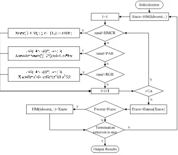
Based on the proposed HS algorithm with the chaotic local search, a hybrid HS with chaos strategy named HSCH is proposed, in which HS is applied to perform global exploration and chaotic local search is employed to perform locally oriented search (exploitation) for the solutions resulted by the HS [23]. The procedure of HSCH is described in Figure 1.

The harmony of worst fitness in the HM needs to be improved. We add chaotic local search to pitch adjusting of HS algorithm. Besides, to maintain population diversity, several new harmony are generated by chaos with certain probability (RGR) and incorporated in the new HM. Thus, the resulting HM members are expected to have better fitness than that of the original ones. This strategy can also overcome the premature shortcoming of the regular HS method. Figure 2 shows the computation procedure of the HSCH Algorithm.

Figure 1. Pseudo Code of the HSCH Algorithm

Figure 2. The flowchart of the HSCH Algorithm.

Procedure HSCH algorithm Initiate_parameters() Initialize_HM()

(1, )

cx



rand

n

, //n denotes the number of variables While (not_termination)

x

new



HM(idworst,:), For i = 1 to n do

If ( rand< HMCR) //memory consideration

Select one harmony from HM randomly:

x

new



x j

j

,



U{1,2,,HMS}; Elseif ( rand< PAR)

new new

,

4

(1

),

2 (

0.5)

i i i

i i i bw

cx

cx

cx

x

x

cx



 











Elseif ( rand < RGR)

new

4

(1

),

(

),

i i i

L U L

i i i i i

cx

cx

cx

x

x

cx

x

x















End End for

Update harmony memory HM // if applicable End while

3. Computational Results and Analysis

In this section we perform some numerical tests in order to illustrate the implementation and efficiency of the proposed method. All the experiments were performed on Windows XP system running on a Hp540 laptop with Intel(R) Core(TM) 2×1.8GHz and 2GB RAM, and the codes were written in MatlabR2010b.

3.1. AVE Problems

AVE 1. Let A be a matrix whose diagonal elements are 500 and the nondiagonal elements are chosen randomly from the interval

[1, 2]

such that A is symmetric. Let

(

)

b



A



I e

where

I

is the identity matrix of order

n

and

e

is n1 vector whose elements are all equal to unity. Since singular values matrix A are all greater than 1, this AVE is uniquely solvable by Lemma 2.2, and the unique solution is

x



(1, 1,



,1)

T.

AVE 2. Let the matrix A is given by , 1 1,

4 ,

,

0,

1, 2,

, .

ii i i i i i j

a



n

a

_



a

_



n

a



i





n

Let b(AI)e where

I

is the identity matrix order

n

and

e

is n1 vector whose elements are all equal to unity. Since singular values matrix A are all greater than 1, this AVE is uniquely solvable by Lemma 2.2, and the unique solution is

(1, 1,

,1)

T

x





.

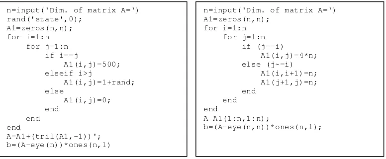
Here the data (A, b) can be generated by following Matlab scripts:

Figure 3. Generating data (A, b) of AVE1 and AVE2 by the Matlab scripts

In AVE1, we set the random-number generator to the state of 0 so that the same data can be regenerated.

AVE 3. Following we consider some randomly generated AVE problem with singular values of

A

exceeding 1 where the data (A, b) are generated by the Matlab scripts:

rand('state',0);

A=rand(n,n)'*rand(n,n)+n*eye(n); b=(A-eye(n,n))*ones(n,1);

Since singular values matrix A are all greater than 1, this AVE is uniquely solvable by Lemma 2.2, and the unique solution is

x



(1, 1,



,1)

T.

3.2. Parameters Setting

Simulations were carried out to compare the optimization (minimization) capabilities of the proposed method (HSCH) with respect to: (a) classical HS (HS,[16]), (b) HSDE [24]. To make the comparison fair, the populations for all the competitor algorithms (for all problems tested) were initialized using the same random seeds. The HS-variants algorithm parameters

n=input('Dim. of matrix A=') rand('state',0);

A1=zeros(n,n); for i=1:n for j=1:n if i==j

A1(i,j)=500; elseif i>j

A1(i,j)=1+rand; else

A1(i,j)=0; end

end end

A=A1+(tril(A1,-1))'; b=(A-eye(n))*ones(n,1)

n=input('Dim. of matrix A=') A1=zeros(n,n);

for i=1:n for j=1:n if (j==i) A1(i,j)=4*n; else (j~=i) A1(i,i+1)=n; A1(j+1,j)=n; end

end end

A=A1(1:n,1:n);

were set the same parameters: harmony memory size HMS=15, harmony memory consideration rate HMCR= 0.6, and the number of improvisations Tmax=10000. In HSCH, RGR is chosen to be 0.2. In classical HS, we set pitch adjusting rate PAR= 0.35. Let the initial point

0

x selected randomly in the given interval [-1,1].

3.3. Results

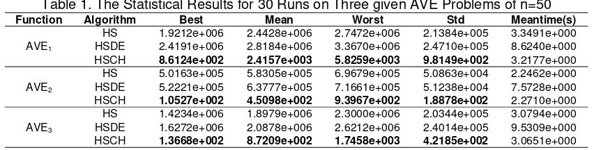
To judge the accuracy of different algorithms, 30 independent runs of each of the three algorithms were carried out and the best, the mean, the worst fitness values, and the standard deviation (Std) were recorded. Table 1 and Table 2 compares the algorithms on the quality of the optimum solution for every AVE problem of n=50 and n=100.

Table 1. The Statistical Results for 30 Runs on Three given AVE Problems of n=50 Function Algorithm Best Mean Worst Std Meantime(s)

AVE1

HS 1.9212e+006 2.4428e+006 2.7472e+006 2.1384e+005 3.3491e+000

HSDE 2.4191e+006 2.8184e+006 3.3670e+006 2.4710e+005 8.6240e+000

HSCH 8.6124e+002 2.4157e+003 5.8259e+003 9.8149e+002 3.2177e+000

AVE2

HS 5.0163e+005 5.8305e+005 6.9679e+005 5.0863e+004 2.2462e+000

HSDE 5.2221e+005 6.3777e+005 7.1661e+005 5.1238e+004 7.5728e+000

HSCH 1.0527e+002 4.5098e+002 9.3967e+002 1.8878e+002 2.2710e+000

AVE3

HS 1.4234e+006 1.8979e+006 2.3000e+006 2.0344e+005 3.0794e+000

HSDE 1.6272e+006 2.0878e+006 2.6212e+006 2.4014e+005 9.5309e+000

HSCH 1.3668e+002 8.7209e+002 1.7458e+003 4.2185e+002 3.0651e+000

Table 2. The Statistical Results for 30 Runs on Three given AVE Problems of n=100 Function Algorithm Best Mean Worst Std Meantime(s)

AVE1

HS 8.7139e+006 9.8264e+006 1.1049e+007 5.6466e+005 8.3361e+000

HSDE 9.4194e+006 1.0785e+007 1.1997e+007 6.5037e+005 2.3022e+001

HSCH 1.8661e+005 2.5579e+005 3.9843e+005 4.9279e+004 8.4083e+000

AVE2

HS 7.1403e+006 8.0176e+006 8.6583e+006 3.9421e+005 6.8993e+000

HSDE 7.7324e+006 8.6878e+006 9.5392e+006 4.8861e+005 2.1845e+001

HSCH 1.3697e+005 2.0031e+005 2.6792e+005 3.5899e+004 6.5297e+000

AVE3

HS 9.4440e+007 1.0742e+008 1.1928e+008 5.5482e+006 1.1561e+001

HSDE 9.6570e+007 1.1399e+008 1.2838e+008 7.6645e+006 2.3033e+001

HSCH 5.6216e+005 9.9070e+005 1.4030e+006 2.2014e+005 1.1020e+001

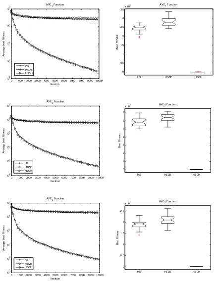
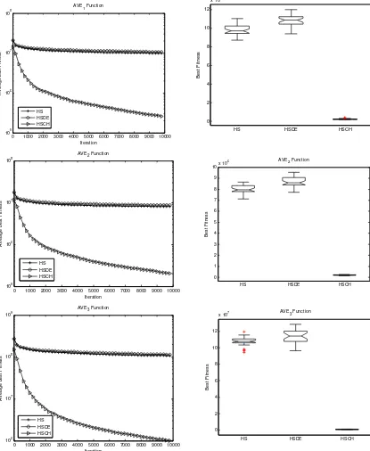
Figure 4 and Figure 5 show the convergence and its boxplot of the best fitness in the population for the different algorithms (HSCH, HS, HSDE) for every AVE problem of n=50 and n=100. The values plotted for every generation are averaged over 30 independent runs. The boxplot is the best fitness in the final population for the different algorithms (HSCH, HS, HSDE) for corresponding AVE problem.

3.4. Analysis

We can see that in all instances the HSCH algorithm performs extremely well, and finally converges to the unique solution of the AVE.The behavior of the two former algorithms (HS and HSDE) is similar for all given AVE problems. From the computation results, the HSDE algorithm is clearly the worst algorithm for all given AVE problems, while the HSCH algorithm is the best.

4. Conclusion

We have proposed HSCH algorithm for solving absolute value equation Ax -|x| = b

by using HSCH approaches. Future works will also focus on studying the applications of HSCH on engineering optimization problems.

Figure 4. The convergence and boxplot of the best fitness for given AVE problems of n=50

0 1000 2000 3000 4000 5000 6000 7000 8000 9000 10000 103 104 105 106 107 Iteration A v erage be s t F it nes s

AVE₁ Function

HS HSDE HSCH 0 0.5 1 1.5 2 2.5 3 3.5

x 106

HS HSDE HSCH

B e s t F it nes s

AVE₁ Function

0 1000 2000 3000 4000 5000 6000 7000 8000 9000 10000 102 103 104 105 106 107 Iteration A v e rage bes t F it ne s s

AVE₂ Function

HS HSDE HSCH 0 1 2 3 4 5 6 7

x 105

HS HSDE HSCH

Be s t F itn e s s AVE 2 Function

0 1000 2000 3000 4000 5000 6000 7000 8000 9000 10000 102 103 104 105 106 107 Iteration A v e rage bes t F it ne s s

AVE₃ Function

HS HSDE HSCH 0 0.5 1 1.5 2 2.5

x 106

HS HSDE HSCH

Be s t F itn e s s

Figure 5. The convergence and boxplot of the best fitness for given AVE problems of n=100

Acknowledgments

This work is supported by National Natural Science Foundation of China under Grant No.60974082, Scientific Research Program Funded by Shaanxi Provincial Education Department under Grant No. 12JK0863, 11JK1066, and Innovation Foundation of Graduate Student by Xidian University under Grant No. K50513100004.

0 1000 2000 3000 4000 5000 6000 7000 8000 9000 10000 105 106 107 108 Iteration A v er age be s t F it ne s s AVE 1 Function

HS HSDE HSCH 0 2 4 6 8 10 12

x 106

HS HSDE HSCH

B e s t F itn e s s

AVE₁ Function

0 1000 2000 3000 4000 5000 6000 7000 8000 9000 10000 105 106 107 108 Iteration A v erage be s t F it nes s

AVE₂ Function

HS HSDE HSCH 0 1 2 3 4 5 6 7 8 9 10x 10

6

HS HSDE HSCH

B es t F it nes s

AVE₂ Function

0 1000 2000 3000 4000 5000 6000 7000 8000 9000 10000 106 107 108 109 Iteration A v e rage bes t F it ne s s

AVE₃ Function

HS HSDE HSCH 0 2 4 6 8 10 12

x 107

HS HSDE HSCH

References

[1] Jiri Rohn. A Theorem of the Alternatives for the Equation Ax+B|x|=b. Linear and Multilinear Algebra, 2004,52 (6):421-426.

[2] Mangasarian O.L. Absolute value programming. Computational Optimization and Aplications, 2007, 36(1): 43-53.

[3] R. W. Cottle and G. Dantzig. Complementary pivot theory of mathematical programming.

Linear Algebra and its Applications. 1968,1:103-125.

[4] Mangasarian O.L., Meyer, R.R. Absolute value equations. Linear Algebra and its Applications, 2006, 419(5): 359-367.

[5] Oleg Prokopyev. On equivalent reformulations for absolute value equations. Computational Optimization and Applications, 2009, 44(3): 363-372.

[6] Shen-Long Hu, Zheng-Hai Huang. A note on absolute value equations. Optim. Lett.2010, 4(3): 417-424.

[7] Mangasarian O.L. Absolute value equation solution via concave minimization. Optim. Lett. 2007, 1(1): 3-8.

[8] Mangasarian O.L. A generlaized newton method for absolute value equations. Optim. Lett. 2009, 3(1): 101-108.

[9] Mangasarian, O.L. Knapsack feasibility as an absolute value equation solvable by successive linear programming. Optim. Lett. 2009, 3(2):161-170.

[10] C. Zhang,Q. J. Wei. Global and Finite Convergence of a Generalized Newton Method for

Absolute Value Equations. Journal of Optimization Theory and Applications. 2009(143):391-403.

[11] Louis Caccetta, Biao Qu, Guanglu Zhou. A globally and quadratically convergent method for

absolute value equations. Computational Optimization and Applications. 2011, 48(1): 45-58.

[12] Longquan Yong, Sanyang Liu, Shemin Zhang and Fang'an Deng. A New Method for

Absolute Value Equations Based on Harmony Search Algorithm. ICIC Express Letters, Part B: Applications, 2011,2(6):1231-1236.

[13] Longquan Yong, Shouheng Tuo. Quasi-Newton Method to Absolute Value Equations based

on Aggregate Function. Journal of Systems Science and Mathematical Sciences,2012,32(11):1427-1436.

[14] Longquan Yong, Sanyang Liu,Zhang Jian-ke,Chen Tao,Deng Fang-an. A New Feasible

Interior Point Method to Absolute Value Equations.Journal of Jilin University (Science Edition), 2012, 50 (5):887-891.

[15] Longquan Yong. An Iterative Method for Absolute Value Equations Problem. Information,

2013,16(1):7-12.

[16] Geem Z W, Kim J H, Loganathan G V. A new heuristic optimization algorithm: harmony

search. Simulation, 2001,76: 60-68.

[17] Lee K S, Geem Z W. A new meta-heuristic algorithm for continuous engineering

optimization: harmony search theory and practice. Computer Methods in Applied Mechanics and Engineering, 2005,194: 3902-3933.

[18] Lakshmi Ravi, S.G. Bharathi dasan.PSO based Optimal Power Flow with Hybrid Distributed

Generators and UPFC.Telkomnika,2012,10(3).

[19] Andi Muhammad Ilyas, M. Natsir Rahman. Economic Dispatch Thermal Generator Using

Modified Improved Particle Swarm Optimization.Telkomnika,2012,10(3): 459-470.

[20] Osama Alia, Rajeswari Mandava.The variants of the harmony search algorithm: an

overview. Artificial Intelligence Review, 2011,36: 49-68.

[21] Swagatam Das, Arpan Mukhopadhyay, Anwit Roy, Ajith Abraham, Bijaya K. Panigrahi.

Exploratory Power of the Harmony Search Algorithm: Analysis and Improvements for Global Numerical Optimization. IEEE Transactions On Systems, Man, and Cybernetics, Part B: Cybernetics, 2011,41:89-106.

[22] Mohammed Azmi Al-Betar, Iyad Abu Doush, Ahamad Tajudin Khader, Mohammed A.

Awadallah. Novel selection schemes for harmony search. Applied Mathematics and Computation, 2012, 218:6095-6117.

[23] Shouheng Tuo, Longquan Yong. Improved Harmony Search Algorithm with Chaos.Journal

of Computational Information Systems,2012,8 (10) : 4269- 4276.

[24] Prithwish Chakraborty,Gourab Ghosh Roy, Swagatam Das, Dhaval Jain, Ajith Abraham. An